Dec 04, 2025 | 445 words | 4 min read
10.3.1. Task 1#
Image Analysis#
Learning Objectives:#
Utilize file I/O functions in Python to handle image data using modern Python libraries.
Analyze image properties such as color composition using manual looping methods.
Develop an understanding of Python libraries for image processing.
Write analysis results to a text file.
Introduction#
Most digital images store color using non-linear values called \(R'G'B'\) (sRGB). In an 8-bit image, each channel (\(R\), \(G\), \(B\)) is stored as an integer from \(0\) to \(255\). These values are gamma-encoded, which makes them efficient for display and storage but unsuitable for precise calculations such as computing brightness or comparing colors. To process the image, we first normalize the values by dividing by \(255.0\), giving floating-point numbers between \(0.0\) and \(1.0\). Next, we linearize these normalized \(R'G'B'\) values to remove the gamma encoding. This is done using the transfer function shown in (10.2), where \(C\) represents one of the three color channels (\(R\), \(G\), or \(B\)). The function applies one formula for darker values and another for brighter ones. For more background, see the sRGB article on Wikipedia.
Task Instructions#
Develop a Python program that computes the average intensity of each channel in an image, and writes the results to a file.
Before creating the program, create a flowchart of the algorithm you will use and save
it as py4_ind_1_username.pdf. Then start
your program from a copy of the
ENGR133_Python_Template.py
Python template. Your program should be named
py4_ind_1_username.py. Your program
should do the following:
Load the user specified image using
PIL.image.open.Convert the image to a NumPy array for easier manipulation. See the official docs for usage details.
Normalize the image’s pixel values to the range \(0\)–\(1\) by dividing each value by \(255.0\). This is necessary for the subsequent linearization calculations.
Linearize the pixels in the image by applying the transformation in (10.2). When applying the transformation, the
ndimattribute may be useful for determining if the image is grayscale or color. See the official docs for usage details.Analyze the color content in the image by computing the mean of the linearized color channels. If the image is grayscale, the mean of should be reported as zero.
The red channel can be accessed using
image[:, :, 0]The green channel can be accessed using
image[:, :, 1]The blue channel can be accessed using
image[:, :, 2]
Write the color analysis results into a text file named color_analysis.txt.
Images |
Download Link |
|---|---|
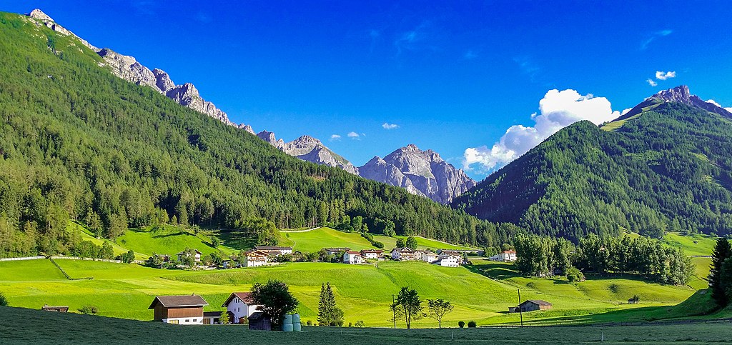
RGB image |
|
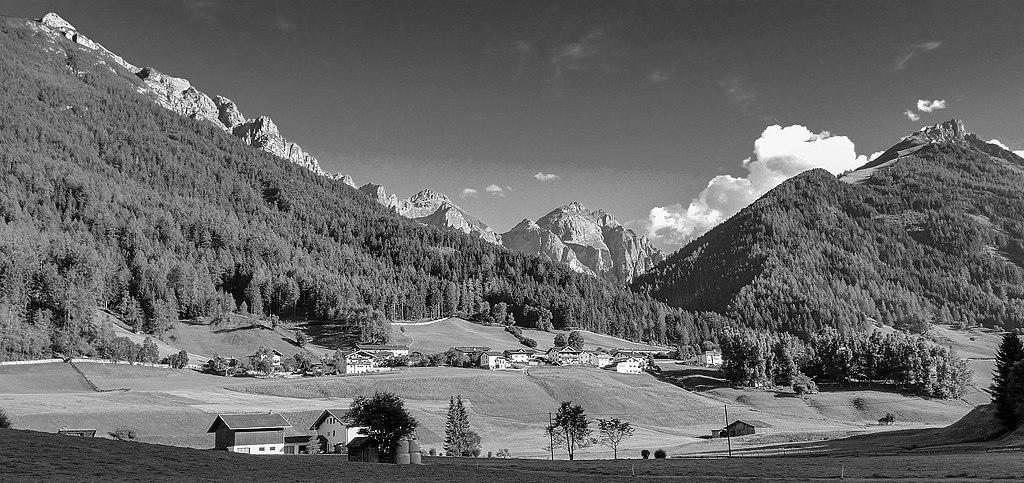
Grayscale image |
Sample Output#
Test cases for the image processing and histogram generation. Use the values in Table 10.8 below to test your program.
Case |
image directory |
|---|---|
1 |
color_image.jpeg |
2 |
grayscale_image.jpeg |
Ensure your program’s output matches the provided samples exactly. This includes all characters, white space, and punctuation. In the samples, user input is highlighted like this for clarity, but your program should not highlight user input in this way.
Case 1 Sample Output
$ python3 py4_ind_1_username.py Enter the filename of the image: color_image.jpeg Color analysis results written to color_analysis.txt
1Image: color_image.jpeg
2Red Channel Mean: 0.13
3Green Channel Mean: 0.22
4Blue Channel Mean: 0.33
Case 2 Sample Output
$ python3 py4_ind_1_username.py Enter the filename of the image: grayscale_image.jpeg Color analysis results written to color_analysis.txt
1Image: grayscale_image.jpeg
2Red Channel Mean: 0.00
3Green Channel Mean: 0.00
4Blue Channel Mean: 0.00
Deliverables |
Description |
|---|---|
py4_ind_1_username.pdf |
Flowchart(s) for this task. |
py4_ind_1_username.py |
Your completed Python code. |