Task 2

13.1.2. Task 2#

Learning Objectives#

Understand the core concepts behind Decision Tree classifiers, including entropy and information gain
Build a Decision Tree model from scratch using a recursive algorithm
Tune hyperparameters such as max_depth and min_samples_split to prevent overfitting
Visualize model performance and the structure of the resulting tree

Task Instructions#

Save the flowcharts for each of your tasks in tp3_team_2_teamnumber.pdf. You will also need to include these flowcharts in your final report.

In this task, you will implement a Decision Tree classifier. Decision Trees are powerful models that make predictions by learning a series of simple if-else questions about the features and their relation to the labels. Your goal is to build the logic that finds the best questions to ask. Your script will load the CSV feature dataset file that you created previously, split it into training, validation, and testing sets, and tune the model hyperparameters using the validation dataset. Remember to use the dataset containing the features. We have given published it in Section 13.1.1.

You will reuse some functions from the previous task, such as load_dataset and train_val_test_split.

Note

For the functions described below, the order of arguments and outputs matters. Please ask TAs for guidance and explanation.

Step 1: Calculate Entropy Function#

Create a function named calculate_entropy

Arguments:

labels (NumPy array): A 1-dimensional array of class labels.

Returns:

entropy (float): The calculated entropy value.

The function should calculate entropy for a set of labels using the formula:

(13.1)#\[E = -\sum_{i=1}^{c}p_{i}\log_{2}(p_{i})\]

Where $p_i$ is the proportion (fraction) of class $i$ appearing in the labels and $c$ is the total count of distinct labels in the set. That is, if a set contains [0,0,1,0,1], there are two distinct labels with proportions $\frac{3}{5}$ and $\frac{2}{5}$. You’ll need to count the occurrences of each unique label to find these proportions.

Step 2: Information Gain Function#

Create a function named information_gain that calculates the information gain from a particular split

Arguments:

parent_labels (NumPy array): an array of parent labels
left_labels (NumPy array): an array of labels in the left child
right_labels (NumPy array): an array of labels in the right child

Returns:

information_gain (float): The information gained by making this split.

This function should calculate information gain using the formulas below. Make sure you use the calculate_entropy function you wrote previously.

Let $S$ be the parent set of labels (pre-split) with entropy $H(S) = -\sum_{i=1}^{c}p_{i}\log_{2}(p_i)$ (as described in the previous function)

Additionally:

$n_S$ is the total number of samples
$n_L, n_R$ are the sizes of the left and right child sets such that $n_L + n_R = n_S$
The class distribution in each subset is determined by counts.

The entropy after a split into subsets $L$ and $R$ is:

$H(S | L, R) = w_L \cdot H(L) + w_R \cdot H(R)$

Where:

$H(S | L, R)$ is the weighted entropy after the split
$H(L), H(R)$ are the entropies of the left and right subsets
$w_L, w_R$ are the weights of the left and right subsets:
$w_L = \frac{n_L}{n_S}$
$w_R = 1 - w_L = \frac{n_R}{n_S}$

The information gained from splitting $S$ into $L$ and $R$ is:

(13.2)#\[IG(S, L, R) = H(S) - H(S | L, R)\]

Expanded form for the split:

(13.3)#\[IG(S, L, R) = -\sum_{i=1}^{c_S} p_i \log_2(p_i) + w_L \cdot \sum_{i=1}^{c_L} q_{Li} \log_2(q_{Li}) + w_R \cdot \sum_{i=1}^{c_R} q_{Ri} \log_2(q_{Ri})\]

Where:

$p_i = \frac{c_{S_i}}{n_S}; c_{S_i}$ is the count of class $i$ in parent set of labels $S$
$q_{Li} = \frac{c_{L_i}}{n_L}; c_{L_i}$ is the count of class $i$ in the left split set $L$
$q_{Ri} = \frac{c_{R_i}}{n_R}; c_{R_i}$ is the count of class $i$ in the right split set $R$

An example calculation of information gain has been provided below.

Example

Let’s say we have a set of 10 labels (e.g., 0 for ‘Stop Sign’, 1 for ‘Right Turn’) and we want to test how much information we gain by performing a specific split.

1. Define the inputs:

parent_labels ($S$) = [0, 0, 1, 0, 1, 0, 0, 1, 0, 1]
left_labels ($L$) = [0, 0, 0, 0, 0, 1]
right_labels ($R$) = [1, 1, 0, 1]

2. Calculate Parent Entropy $H(S)$:

Total samples $n_S = 10$
Counts in $S$: 6 (Class 0), 4 (Class 1)
Proportions: $p_0 = 6/10 = 0.6$, $p_1 = 4/10 = 0.4$
Entropy $H(S) = - [ (0.6 \cdot \log_2(0.6)) + (0.4 \cdot \log_2(0.4)) ]$ $H(S) = - [ (0.6 \cdot -0.737) + (0.4 \cdot -1.322) ]$ $H(S) = - [ -0.4422 - 0.5288 ] = -(-0.971) = \mathbf{0.971}$

3. Calculate Child Entropies $H(L)$ and $H(R)$:

Left Child $H(L)$:
- Total samples $n_L = 6$
- Counts in L: 5 (Class 0), 1 (Class 1)
- Proportions: $p_0 = 5/6 \approx 0.833$, $p_1 = 1/6 \approx 0.167$
- $H(L) = - [ (0.833 \cdot \log_2(0.833)) + (0.167 \cdot \log_2(0.167)) ]$ $H(L) = - [ (0.833 \cdot -0.263) + (0.167 \cdot -2.585) ]$ $H(L) = - [ -0.219 - 0.431 ] = -(-0.650) = \mathbf{0.650}$
Right Child $H(R)$:
- Total samples $n_R = 4$
- Counts in R: 1 (Class 0), 3 (Class 1)
- Proportions: $p_0 = 1/4 = 0.25$, $p_1 = 3/4 = 0.75$
- $H(R) = - [ (0.25 \cdot \log_2(0.25)) + (0.75 \cdot \log_2(0.75)) ]$ $H(R) = - [ (0.25 \cdot -2.0) + (0.75 \cdot -0.415) ]$ $H(R) = - [ -0.5 - 0.311 ] = -(-0.811) = \mathbf{0.811}$

4. Calculate Weighted Entropy $H(S | L, R)$:

Weights: $w_L = n_L / n_S = 6 / 10 = 0.6$, $w_R = n_R / n_S = 4 / 10 = 0.4$
$H(S | L, R) = (w_L \cdot H(L)) + (w_R \cdot H(R))$ $H(S | L, R) = (0.6 \cdot 0.651) + (0.4 \cdot 0.811)$ $H(S | L, R) = 0.3906 + 0.3244 = \mathbf{0.715}$

5. Calculate Information Gain $IG(S, L, R)$:

$IG = H(S) - H(S | L, R)$
$IG = 0.971 - 0.715 = \mathbf{0.256}$

This split reduced the entropy (uncertainty) from 0.971 to 0.715, giving us an Information Gain of 0.256. The algorithm would repeat this process for all possible splits and choose the one with the highest information gain.

Note

Ensure that you understand what entropy is and how it relates to the information gain. Pondering the following questions will help.

What do you think the entropy of an array of labels is if it only contains one class? (only stop signs)

Does it make sense to split an array if it only contains stop sign labels? Would such a split give you any information gain?

What kind of split would get you the most information gain.

Step 3: Find the Best Split#

Create a function named find_best_split that iterates through the feature columns to find the one that best separates the data and at what threshold.

Arguments:

X (NumPy array): an array of features
y (NumPy array): an array of labels

Returns:

best_feature (int): the index of the best feature column to split on
best_threshold (float): The threshold value for the best split
best_gain (float): the information gain of the best split

For each feature, you need to find the best threshold to split it. A common technique is to use the midpoint between each pair of unique sorted values as potential thresholds and iterate among them. You may find the np.unique() function useful for this as it returns the sorted unique values in an array.

For each potential split, calculate the information gain. You may find the split_dataset function provided below useful for dividing the dataset into left and right subsets based on a feature index and threshold. Keep track of the split that results in the highest gain as that will be the best split. Finally, return the feature index and split threshold that yields the highest information gain.

Code Snippet: The function below demonstrates how to perform a split. It will be handy to test every potential split to find out which yields the highest information gain.

def split_dataset(X, y, feature_index, threshold):
 """
 Splits a dataset based on a feature and threshold.
 """
 X_left, y_left, X_right, y_right = [], [], [], []

 for i, example in enumerate(X):
     if example[feature_index] < threshold:
         X_left.append(example)
         y_left.append(y[i])
     else:
         X_right.append(example)
         y_right.append(y[i])

 return np.array(X_left), np.array(y_left), np.array(X_right), np.array(y_right)

Step 4: Build the Decision Tree#

Create a function named build_decision_tree. This is the core of the classifier and will be recursive, that is, it will call itself.

Arguments:

X (NumPy array): an array of features at the current node
y (NumPy array): an array of corresponding labels at the current node
max_depth (int): The maximum depth the tree is allowed to grow to
min_samples_split (int): the minimum number of samples required to split a node
current_depth (int): the current depth of the node in the tree

Returns:

tree (dict): A dictionary representing the left or right subtree or a leaf node

Use the following structure for the tree dictionary if it represents a subtree.

  tree = {
    "feature": best_feature_index,
    "threshold": best_threshold_value,
    "left": left_subtree,
    "right": right_subtree
  }

Use the following structure for the tree dictionary if it represents a leaf node.

  tree = {"label": predicted_label}

Note

The keys in the dictionary must match the ones shown below. The values contain placeholder variables in the examples above that you must calculate.

The idea here is that to make a prediction for a new image using a decision tree, you will follow the tree splits for its features based on the determined thresholds until you reach a leaf node which contains a prediction for what label the image likely is.

This function will recursively build the tree. To ensure that the function does not keep calling itself forever, you must define the following stopping conditions (base cases) for the recursion:

If all labels in a node are the same, it becomes a leaf node predicting that label.
If max_depth is reached or the number of samples is less than min_samples_split, it becomes a leaf node predicting the most common label.
If no split provides a positive information gain, it also becomes a leaf node.

If none of these stopping conditions are met, find the best split using find_best_split, split the dataset accordingly into X_left, y_left, X_right, y_right. Then, recursively call build_decision_tree to build the left and right subtrees.

Note

We highly recommend asking a TA for help with this function as recursion is a fundemental but tricky programming concept.

Step 5: Make Predictions#

Create a function named predict that uses a trained decision tree to predict labels for a dataset.

Arguments:

tree (dict): The trained decision tree
X (NumPy array): an array of image features to predict labels for

Returns:

predicted_labels (NumPy array): An array of predicted labels

It’s helpful to first create a helper function, predict_single(tree, x), that traverses the tree for a single data point’s 1D feature array x.

The predict function can then loop through all rows in X and call predict_single on each row. This would be similar to what you did in Step 5: KNN Individual Prediction and Step 6: KNN Prediction Function.

Step 6: Hyperparameter Tuning and Plotting#

This task involves tuning two hyperparameters: max_depth and min_samples_split. You will create two functions to tune them separately and a plotting function to visualize the results.

Create two functions, tune_max_depth and tune_min_samples_split. Each function should:

Loop through a predefined list of values for its respective hyperparameter.
For each value, build a decision tree using the training data.
Calculate the accuracy on both the training and validation sets.
After the loop, call plot_dt_performance to display the results.

Arguments for tune_max_depth:

X_train (NumPy array): an array of training image features
y_train (NumPy array): an array of training image labels
X_val (NumPy array): an array of validation image features
y_val (NumPy array): an array of validation image labels

Arguments for tune_min_samples_split:

X_train (NumPy array): an array of training image features
y_train (NumPy array): an array of training image labels
X_val (NumPy array): an array of validation image features
y_val (NumPy array): an array of validation image labels
max_depth (int): the optimal max_depth as determined by the user after running the previous tuning function

Note that the arguments for both are not expected to return anything. When testing the max depth values with the tune_max_depth function, use min_samples_split = 2 for all trees.

Below you can find some helpful starter code for the plotting function. Note that you will need to modify it to ensure that your plots match the examples given below.

  def plot_dt_performance(train_accs, val_accs, param_values, param_name):
    """
    Generates a plot to visualize hyperparameter tuning performance.
    """
    fig, axes = plt.subplots(1, 1, figsize=(8, 6))
    axes.plot(param_values, train_accs, marker='x', label='Training Accuracy')
    axes.plot(param_values, val_accs, marker='x', label='Validation Accuracy')
    axes.set_xlabel(param_name)
    axes.set_ylabel('Accuracy')

    plt.tight_layout()
    plt.show()

Step 7: Main Function#

Create a main function that collects the following input from the user:

The path of the csv file containing the feature dataset
The optimal max depth according to the user’s interpretation of the tuning plot
The optimal min samples split according to the user’s interpretation of the tuning plot

The function should:

Load the dataset using the function from Step 1: Load Dataset Function. You will need to pass in the feature column names and the label column name as you did in the previous task Section 13.1.1.
Split the dataset into train, validation and test sets. A ‘set’ is a pair of X (feature array) and corresponding y (the labels). You can use the function you created in Step 2: Train-Validation-Test Split Function.
Display the sizes of the Training, Validation, and Test sets.
Call the tune_max_depth function to test the sample values [1, 2, 3, 4, 5, 7, 10, 15].
Call the tune_min_samples_split function to test the sample values [1, 2, 3, 4, 5, 7, 10, 15].
Ask the user to assess the optimal values for the hyperparameters using the graphs showing how training and validation accuracy varies with each hyperparameter.

Bonus

How do you think the optimal values for the hyperparameters should be determined?

Why didn’t we scale the feature dataset?

Is a more complex tree (deeper tree with fewer samples in the leaves) better?

Build the final decision tree using the training set and the user-provided optimal hyperparameters
Calculate and display the final model’s accuracy on the training, validation, and test sets.
Use the print function below to display what the tree looks like.

Hints on saving time when debugging

You may find the function below useful for printing the tree as you go to see if the splits you are making make sense.

  def print_tree(tree, feature_names, indent=""):
    """
    Recursively prints the decision tree in a readable format.
    """
    # Base case: we have reached a leaf node
    if "label" in tree:
        # Map the numeric label to a meaningful name
        label_name = "Stop Sign" if tree["label"] == 0 else "Right Turn Sign"
        print(f"{indent}Predict: {label_name}")
        return

    # Extract information for the current decision node
    feature_index = tree["feature"]
    feature_name = feature_names[feature_index]
    threshold = tree["threshold"]

    rule = f"{feature_name} < {threshold:.2f}"

    # Recursively print the 'true' branch (left)
    print(f"{indent}If {rule}:")
    print_tree(tree["left"], feature_names, indent + "  ")

    # Recursively print the 'false' branch (right)
    print(f"{indent}Else ({rule.replace('<', '>')})")
    print_tree(tree["right"], feature_names, indent + "  ")

Ensure that your outputs match the examples below.

Save your program as tp3_team_2_teamnumber.py.

Sample Output#

Use the values in Table 13.5 below to test your program.

Table 13.5 Test Cases#
Case	dataset	optimal_max_depth	optimal_min_samples_split
1	img_features.csv	3	30
2	img_features.csv	7	3

Ensure your program’s output matches the provided samples exactly. This includes all characters, white space, and punctuation. In the samples, user input is highlighted like this for clarity, but your program should not highlight user input in this way.

Case 1 Sample Output

$ python3 tp3_team_2_teamnumber.py Enter the path to the feature dataset: img_features.csv

Data loaded and split: Training set: size: 1175 Validation set: size: 147 Test set: size: 147

Finding optimal tree max depth and min samples split...

Enter the optimal max depth according to your interpretation of the plot: 3 Enter the optimal min samples split according to your interpretation of the plot: 30 Evaluating final model on test set with the chosen hyperparameters

--- Final Model Performance --- Test Set Accuracy: 0.7619 Validation Set Accuracy: 0.7143 Training Set Accuracy: 0.8919

--- Final Decision Tree Rules --- If hue_mean < 61.62: If hue_mean < 54.34: Predict: Stop Sign Else (hue_mean > 54.34) If num_lines < 20.00: Predict: Stop Sign Else (num_lines > 20.00) Predict: Stop Sign Else (hue_mean > 61.62) If hue_std < 82.37: If hue_std < 74.72: Predict: Right Turn Sign Else (hue_std > 74.72) Predict: Right Turn Sign Else (hue_std > 82.37) If num_lines < 38.50: Predict: Stop Sign Else (num_lines > 38.50) Predict: Stop Sign

Fig. 13.3 Case_1_dt_tuning_Max_Depth.png#

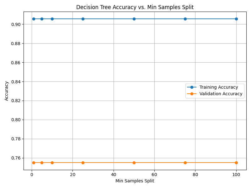
Fig. 13.4 Case_1_dt_tuning_Min_Samples_Split.png#

Case 2 Sample Output

$ python3 tp3_team_2_teamnumber.py Enter the path to the feature dataset: img_features.csv

Data loaded and split: Training set: size: 1175 Validation set: size: 147 Test set: size: 147

Finding optimal tree max depth and min samples split...

Enter the optimal max depth according to your interpretation of the plot: 7 Enter the optimal min samples split according to your interpretation of the plot: 3 Evaluating final model on test set with the chosen hyperparameters

--- Final Model Performance --- Test Set Accuracy: 0.7687 Validation Set Accuracy: 0.8435 Training Set Accuracy: 0.9762

--- Final Decision Tree Rules --- If hue_mean < 61.62: If hue_mean < 54.34: Predict: Stop Sign Else (hue_mean > 54.34) If num_lines < 20.00: If saturation_mean < 109.40: If saturation_mean < 95.37: Predict: Right Turn Sign Else (saturation_mean > 95.37) If value_std < 41.26: Predict: Stop Sign Else (value_std > 41.26) Predict: Stop Sign Else (saturation_mean > 109.40) Predict: Right Turn Sign Else (num_lines > 20.00) Predict: Stop Sign Else (hue_mean > 61.62) If hue_std < 82.37: If hue_std < 74.72: Predict: Right Turn Sign Else (hue_std > 74.72) If saturation_mean < 103.60: If saturation_std < 75.10: Predict: Stop Sign Else (saturation_std > 75.10) If hue_mean < 62.54: Predict: Stop Sign Else (hue_mean > 62.54) Predict: Right Turn Sign Else (saturation_mean > 103.60) If hue_mean < 130.00: If num_lines < 47.50: Predict: Right Turn Sign Else (num_lines > 47.50) Predict: Right Turn Sign Else (hue_mean > 130.00) Predict: Stop Sign Else (hue_std > 82.37) If num_lines < 38.50: If hue_std < 87.13: If value_std < 10.59: Predict: Right Turn Sign Else (value_std > 10.59) If has_circle < 0.50: If value_mean < 47.28: Predict: Right Turn Sign Else (value_mean > 47.28) Predict: Stop Sign Else (has_circle > 0.50) Predict: Right Turn Sign Else (hue_std > 87.13) If hue_mean < 131.46: If saturation_mean < 118.38: If num_lines < 10.50: Predict: Right Turn Sign Else (num_lines > 10.50) Predict: Stop Sign Else (saturation_mean > 118.38) If value_std < 48.45: Predict: Stop Sign Else (value_std > 48.45) Predict: Right Turn Sign Else (hue_mean > 131.46) If saturation_std < 79.59: Predict: Right Turn Sign Else (saturation_std > 79.59) Predict: Stop Sign Else (num_lines > 38.50) If saturation_mean < 141.93: If hue_mean < 122.07: If saturation_mean < 70.20: If hue_std < 87.53: Predict: Right Turn Sign Else (hue_std > 87.53) Predict: Stop Sign Else (saturation_mean > 70.20) Predict: Stop Sign Else (hue_mean > 122.07) Predict: Right Turn Sign Else (saturation_mean > 141.93) Predict: Right Turn Sign

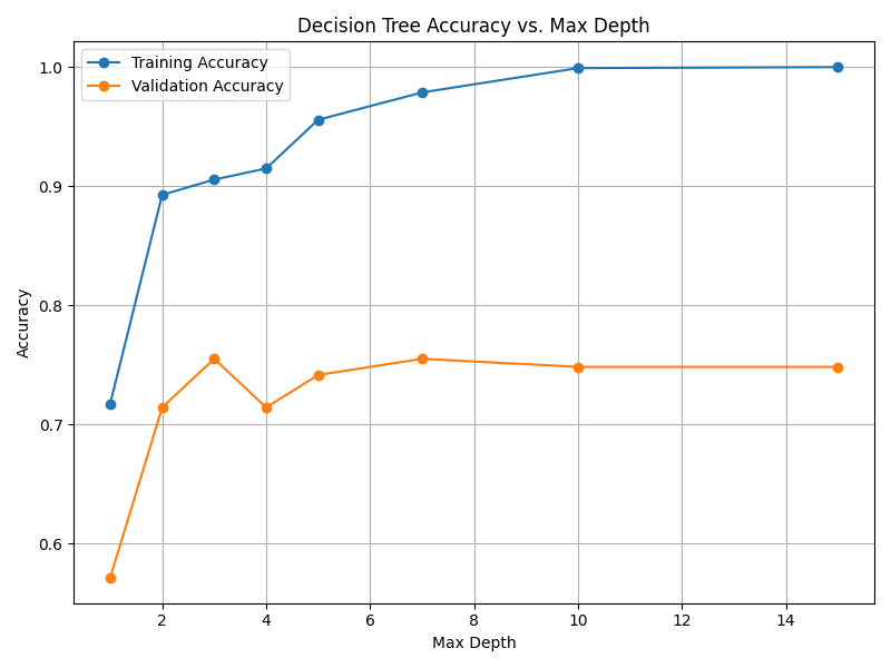
Fig. 13.5 Case_2_dt_tuning_Max_Depth.png#

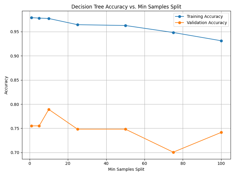
Fig. 13.6 Case_2_dt_tuning_Min_Samples_Split.png#

Table 13.6 Deliverables#
Deliverables	Description
tp3_team_2_teamnumber.pdf	Flowchart(s) for this task.
tp3_team_2_teamnumber.py	Your completed Python code.

Task 2

Contents

13.1.2. Task 2#

Learning Objectives#

Task Instructions#

Step 1: Calculate Entropy Function#

Step 2: Information Gain Function#

Step 3: Find the Best Split#

Step 4: Build the Decision Tree#

Step 5: Make Predictions#

Step 6: Hyperparameter Tuning and Plotting#

Step 7: Main Function#

Sample Output#