\[ \begin{align}\begin{aligned}\newcommand\blank{~\underline{\hspace{1.2cm}}~}\\% Bold symbols (vectors) \newcommand\bs[1]{\mathbf{#1}}\\% Differential \newcommand\dd[2][]{\mathrm{d}^{#1}{#2}} % use as \dd, \dd{x}, or \dd[2]{x}\\% Poor man's siunitx \newcommand\unit[1]{\mathrm{#1}} \newcommand\num[1]{#1} \newcommand\qty[2]{#1~\unit{#2}}\\\newcommand\per{/} \newcommand\squared{{}^2} \newcommand\cubed{{}^3} % % Scale \newcommand\milli{\unit{m}} \newcommand\centi{\unit{c}} \newcommand\kilo{\unit{k}} \newcommand\mega{\unit{M}} % % Percent \newcommand\percent{\unit{{\kern-4mu}\%}} % % Angle \newcommand\radian{\unit{rad}} \newcommand\degree{\unit{{\kern-4mu}^\circ}} % % Time \newcommand\second{\unit{s}} \newcommand\s{\second} \newcommand\minute{\unit{min}} \newcommand\hour{\unit{h}} % % Distance \newcommand\meter{\unit{m}} \newcommand\m{\meter} \newcommand\inch{\unit{in}} \newcommand\foot{\unit{ft}} % % Force \newcommand\newton{\unit{N}} \newcommand\kip{\unit{kip}} % kilopound in "freedom" units - edit made by Sri % % Mass \newcommand\gram{\unit{g}} \newcommand\g{\gram} \newcommand\kilogram{\unit{kg}} \newcommand\kg{\kilogram} \newcommand\grain{\unit{grain}} \newcommand\ounce{\unit{oz}} % % Temperature \newcommand\kelvin{\unit{K}} \newcommand\K{\kelvin} \newcommand\celsius{\unit{{}^\circ C}} \newcommand\C{\celsius} \newcommand\fahrenheit{\unit{{}^\circ F}} \newcommand\F{\fahrenheit} % % Area \newcommand\sqft{\unit{sq\,\foot}} % square foot % % Volume \newcommand\liter{\unit{L}} \newcommand\gallon{\unit{gal}} % % Frequency \newcommand\hertz{\unit{Hz}} \newcommand\rpm{\unit{rpm}} % % Voltage \newcommand\volt{\unit{V}} \newcommand\V{\volt} \newcommand\millivolt{\milli\volt} \newcommand\mV{\milli\volt} \newcommand\kilovolt{\kilo\volt} \newcommand\kV{\kilo\volt} % % Current \newcommand\ampere{\unit{A}} \newcommand\A{\ampere} \newcommand\milliampereA{\milli\ampere} \newcommand\mA{\milli\ampere} \newcommand\kiloampereA{\kilo\ampere} \newcommand\kA{\kilo\ampere} % % Resistance \newcommand\ohm{\Omega} \newcommand\milliohm{\milli\ohm} \newcommand\kiloohm{\kilo\ohm} % correct SI spelling \newcommand\kilohm{\kilo\ohm} % "American" spelling used in siunitx \newcommand\megaohm{\mega\ohm} % correct SI spelling \newcommand\megohm{\mega\ohm} % "American" spelling used in siunitx % % Capacitance \newcommand\farad{\unit{F}} \newcommand\F{\farad} \newcommand\microfarad{\micro\farad} \newcommand\muF{\micro\farad} % % Inductance \newcommand\henry{\unit{H}} \newcommand\H{\henry} \newcommand\millihenry{\milli\henry} \newcommand\mH{\milli\henry} % % Power \newcommand\watt{\unit{W}} \newcommand\W{\watt} \newcommand\milliwatt{\milli\watt} \newcommand\mW{\milli\watt} \newcommand\kilowatt{\kilo\watt} \newcommand\kW{\kilo\watt} % % Energy \newcommand\joule{\unit{J}} \newcommand\J{\joule} % % Composite units % % Torque \newcommand\ozin{\unit{\ounce}\,\unit{in}} \newcommand\newtonmeter{\unit{\newton\,\meter}} % % Pressure \newcommand\psf{\unit{psf}} % pounds per square foot \newcommand\pcf{\unit{pcf}} % pounds per cubic foot \newcommand\pascal{\unit{Pa}} \newcommand\Pa{\pascal} \newcommand\ksi{\unit{ksi}} % kilopound per square inch \newcommand\bar{\unit{bar}} \end{aligned}\end{align} \]

Dec 04, 2025 | 1684 words | 17 min read

13.1.1. Task 1

Learning Objectives

• Learn how a K-Nearest Neighbors (KNN) Classifier works and build one from scratch

• Load a dataset and split it into training, validation, and testing sets

• Understand what hyperparameters are and how to tune them using a validation set

• Apply feature scaling (standardization) to improve model performance.

Task Instructions

Save the flowcharts for each of your tasks in tp3_team_1_teamnumber.pdf. You will also need to include these flowcharts in your final report.

In this task, you’ll build a K-Nearest Neighbors (KNN) classifier. Your script will load a CSV dataset file that you created previously, split it into training, validation, and testing sets, and tune the model hyperparameters using the validation dataset. Remember to use the dataset containing the features you created in Section 12.2.3.

Note

For the functions described below, the order of arguments and outputs matters. Please ask TAs for guidance and explanation.

Step 1: Load Dataset Function

Create a function named load_dataset

Arguments:

• file_path (str): Path to the CSV file.

• feature_cols (list of str): Names of columns to use as features

• label_col (str): Name of the column containing binary labels (0 or 1)

• shuffle (bool, default True): Whether to shuffle the data.

• seed (int, default 42): Seed for reproducibility

Returns:

• X: a NumPy array of features

• y: a NumPy array of labels

The function must load the CSV file using pandas.read_csv(). Then, extract the feature columns (feature_cols) into array X, and the label column (label_col) into array y. To convert extracted subsets of a Pandas DataFrame into a Numpy array, you can use the .to_numpy() method. If shuffle is True, set the seed using np.random.seed(seed) and generate a shuffled index using np.random.permutation(len(y)). You can use this shuffled index to reorder X and y.

• Code Snippet: The code snippet below demonstrates how to load the dataset. (We are giving it away, but please understand what it does!)

  def load_dataset(file_path, feature_cols, label_col, shuffle, seed=70):
   """
   Loads a dataset from a CSV file, separates features and labels,
   and optionally shuffles the data.
   """
   df = pd.read_csv(file_path)
   X = df[feature_cols].to_numpy()
   y = df[label_col].to_numpy()
  
   if shuffle:
       np.random.seed(seed)
       shuffled_indices = np.random.permutation(len(y))
       X = X[shuffled_indices]
       y = y[shuffled_indices]
  
   return X, y
  

Step 2: Train-Validation-Test Split Function

Create a function named train_val_test_split that splits the data into an 80:10:10 ratio for training, validation, and testing.

Arguments:

• X (NumPy array): an array of image features

• y (NumPy array): an array of image labels

• train_ratio (float): a decimal value indicating the proportion of data for training (default=0.8)

• val_ratio (float): a decimal value indicating the proportion of data for validation (default=0.1)

• test_ratio (float): a decimal value indicating the proportion of data for testing (default=0.1)

Returns:

• X_train: a NumPy array of training features

• y_train: a NumPy array of training labels

• X_val: a NumPy array of validation features

• y_val: a NumPy array of validation labels

• X_test: a NumPy array of testing features

• y_test: a NumPy array of testing labels

This function should ensure that the three ratios sum up to 1. Use the ratios to allocate the rows of the features and labels. For example, if the default ratios are used, simply allocate the first 80% of X rows to X_train & he first 80% of y rows to y_train, the next 10% for validation, the final 10% for testing.

Note

Ensure you do not skip any rows and that the number of rows in train, validation, and test sum up to the number of rows in the original dataset.

Step 3: Feature Scaling Function

Create a function named scale_features that scales the feature data for training, validation, and testing.

Arguments:

• X_train (NumPy array): an array of training image features

• X_val (NumPy array): an array of validation image features

• X_test (NumPy array): an array of testing image features

Returns:

• X_train_scaled (NumPy array): a scaled array of training image features

• X_val_scaled (NumPy array): a scaled array of validation image features

• X_test_scaled (NumPy array): a scaled array of testing image features

The function should calculate the mean and standard deviation of the columns in X_train. Use the mean and standard deviation to scale each column using the formula below:

X_train_scaled = (X_train - mean) / std_dev

Step 4: Metrics Function

Create a function named calculate_metrics that evaluates your model’s prediction by returning the accuracy and error.

Arguments:

• predicted_labels (NumPy array): a 1-dimensional array containing classId predictions

• true_labels (NumPy array): a 1-dimensional array containing the actual classId

Returns:

• accuracy (float): the proportion of correct predictions

• error (float): the proportion of incorrect predictions

The function should compare the predicted labels to the true labels. Accuracy is the fraction of correct predictions. The error rate is 1 - accuracy

Step 5: KNN Individual Prediction

Create a function named knn_single_prediction that predicts the class for a single data point given its features.

Arguments:

• new_example (NumPy array): an array containing the features of a new example for which you want to predict the class

• X_train (NumPy array): an array of training image features

• y_train (NumPy array): an array of training image labels

• k (int): the number of nearest neighbors

Returns:

• predicted_label (int): 0 for stop sign, 1 for right turn

The function should calculate the Euclidean distance from the new_example to every example in X_train using np.linalg.norm(). Find the k training examples with the least distances (the “nearest neighbors”) from the new_example. Determine the most frequent label among those nearest neighbors (this is the “majority vote”). Return this label.

Note

We highly recommend asking a TA for help with this function as there are many ways to reduce the runtime of your code by making this function run efficiently.

Hints on sorting and keeping track of classes

Consider creating a list of distances containing tuples of (distance, ClassId) for each training image. The .sort() method can help you sort this array of tuples according to the distance.

You can then determine the prediction for the new example by selecting the majority class appearing in the first k elements of the sorted distances array.

Step 6: KNN Prediction Function

Create a function named predict_labels_knn that predicts the class for every example in a given dataset of features.

Arguments:

• X_new (NumPy array): The new dataset of image features for which you want to predict the class for each row

• X_train (NumPy array): an array of training image features

• y_train (NumPy array): an array of training image labels

• k (int): the number of nearest neighbours

Returns:

• predicted_labels (NumPy array): an array of predicted labels for the features in X_new

The function should iterate over the rows in X_new and use knn_single_prediction to get the predicted label of each row. Collect these predictions and return them as an array.

Step 7: Hyperparameter Tuning

Create a function named tune_k_values that tests different k values with the validation set to determine the optimal k value to use.

Arguments:

• k_values (list[int]): a list of k values

• X_train (NumPy array): an array of training image features

• y_train (NumPy array): an array of training image labels

• X_val (NumPy array): an array of validation image features

• y_val (NumPy array): an array of validation image labels

• is_shuffle (bool): whether the dataset was shuffled or not

Returns:

• best_k (int): the best value of k for the validation set

The function should iterate through each k in k_values. For each k, predict labels for both the training and validation sets and calculate their accuracy and error rates using predict_labels_knn and calculate_metrics. After the loop, call plot_knn_performance to visualize these metrics.

Return the k value that resulted in the highest validation accuracy. If two values of k both result in the highest validation accuracy, return the lesser one.

Note

For each value of k, append the metrics into a dictionary like this:

metrics = {
        "acc": {"train_acc": [], "val_acc": []},
        "error": {"train_error": [], "val_error": []}
    }

You will need to pass this dictionary to the plotting function in Step 8.

Hint

Once you get to this stage, you may realize that the hyperparameter tuning process is slow, just like the previous task in which you extracted features. This is because during hyperparameter tuning you are running the model for several k values.

Instead of recomputing the metrics every time you run your script, you could save the metrics into a CSV file. Then, in future runs, you can simply load this CSV file directly if it exists. You may find Pathlib useful for checking if a file exists.

This technique is called caching and you may find it useful for future tasks too. If you choose to implement caching (and save yourself time), you will find that you have different metrics for a shuffled dataset versus a non-shuffled dataset. So, make sure to include whether the dataset was shuffled or not in the cache filename using the is_shuffle argument.

Step 8: Plotting Function

To visualize the tuning process, create a function named plot_knn_performance that plots the training and validation curves.

Arguments:

• metrics (dict): See the note above

• k_values (list[int]): the list of k values used to create the metrics dictionary

The function should create a figure with two side-by-side plots: (1) Accuracy vs k and (2) Error Rate vs k. Each plot should show separate lines for training and validation performance. Be sure to include titles, axis labels, and a legend. See the examples and match the formatting.

• Code Snippet: Use the function below as a template.

  def plot_knn_performance(metrics, k_values):
   """
  
   Produces a figure with two plots: Accuracy vs. k and Error Rate vs. k.
   """
   fig, axes = plt.subplots(1, 2, figsize=(15, 6))
  
   # Accuracy Plot
   axes[0].plot(k_values, metrics["acc"]["train_acc"])
   axes[0].plot(k_values, metrics["acc"]["val_acc"])
  
   # Error Rate Plot
   axes[1].plot(k_values, metrics["error"]["train_error"])
   axes[1].plot(k_values, metrics["error"]["val_error"])
  
   plt.tight_layout()
   plt.show()
  

Step 9: Main Function

Create a main function that collects the following inputs from the user:

• The path of the csv file containing the feature dataset

• The choice for shuffling the dataset

• The seed for shuffling the dataset (will be ignored if the user chooses not to shuffle)

The function should then:

1. Load the dataset and shuffle if needed using the function from Step 1: Load Dataset Function. You will need to pass in the feature column names and the label column. You can find the names of the column by viewing the feature dataset CSV file in a text editor or spreadsheet program.

2. Split the dataset into train, validation and test sets. A ‘set’ is a pair of X (feature array) and corresponding y (the labels). You can use the function you created in Step 2: Train-Validation-Test Split Function.

3. Scale the features ensuring that you use the same scaling factors as the training set for all 3 sets. Use the function you wrote for Step 3: Feature Scaling Function.

4. Display the sizes of the Training, Validation, and Test sets.

5. Use the function from Step 7: Hyperparameter Tuning to determine the best value of k among the following:

[1, 9, 20, 40, 80, 130, 200, 300, 500, 750, 1000]

6. Display the graphs showing how training and validation accuracy/error varies with the value of k.

Bonus

Why do you think the training accuracy is 100% for k = 1?

Should we shuffle the dataset to measure the model’s performance? Why?

7. Calculate and display the final model performance on the test set using the previously determined optimal value of k.

Save your program as tp3_team_1_teamnumber.py.

Table 13.2 Feature Dataset

File Name	Description
img_features.csv	Image feature dataset (from previous checkpoint)

Sample Output

Use the values in Table 13.3 below to test your program.

Table 13.3 Test Cases

Case	dataset	shuffle	seed
1	img_features.csv	no	70
2	img_features.csv	yes	70

Ensure your program’s output matches the provided samples exactly. This includes all characters, white space, and punctuation. In the samples, user input is highlighted like this for clarity, but your program should not highlight user input in this way.

Case 1 Sample Output

$ python3 tp3_team_1_teamnumber.py Enter the path to the feature dataset: img_features.csv Shuffle the dataset? (yes/no): no Enter a seed for loading the dataset: 70

Data loaded and split into

Training set: size: 1175 Validation set: size: 147 Test set: size: 147

Based on the plots, the best k appears to be: 200

Evaluating final model on test set with k = 200...

--- Final Model Performance --- Test Set Accuracy: 0.6667 Test Set Error Rate: 0.3333

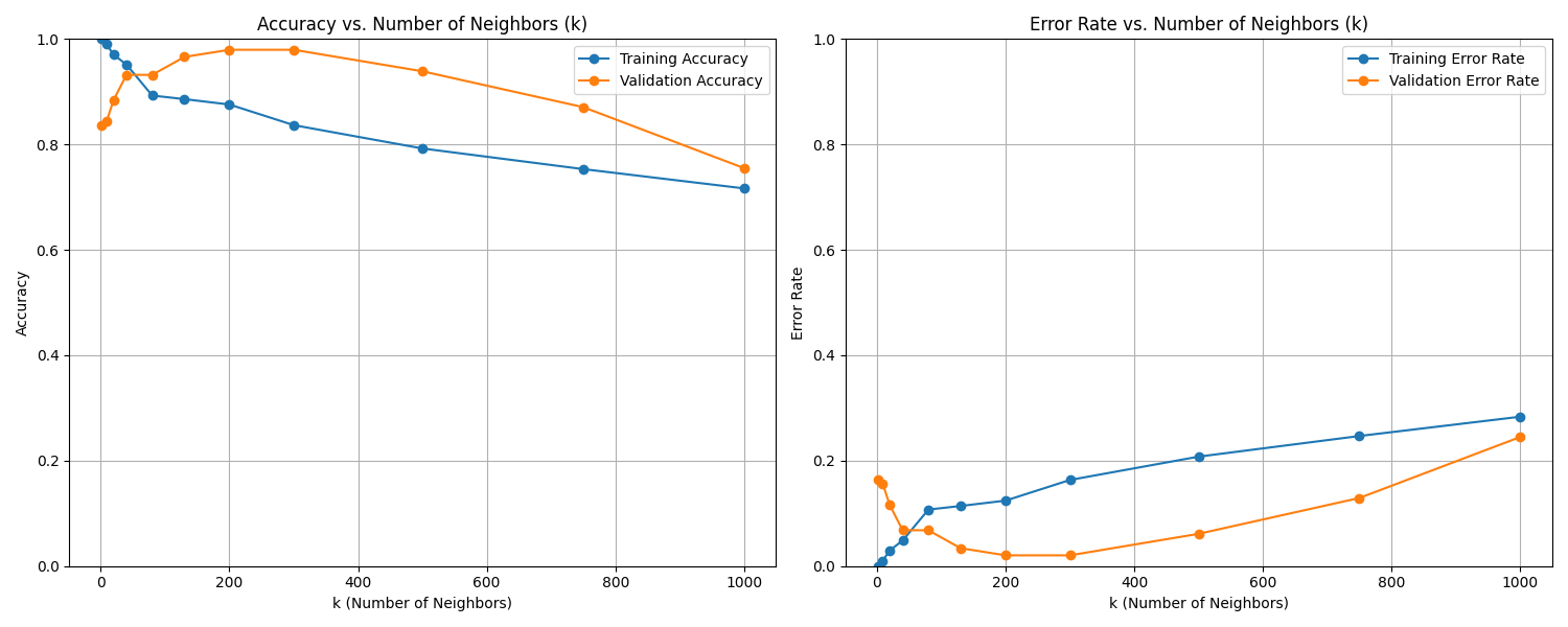
Fig. 13.1 Case_1_train_val.png

Case 2 Sample Output

$ python3 tp3_team_1_teamnumber.py Enter the path to the feature dataset: img_features.csv Shuffle the dataset? (yes/no): yes Enter a seed for loading the dataset: 70

Data loaded and split into

Training set: size: 1175 Validation set: size: 147 Test set: size: 147

Based on the plots, the best k appears to be: 1

Evaluating final model on test set with k = 1...

--- Final Model Performance --- Test Set Accuracy: 0.9728 Test Set Error Rate: 0.0272

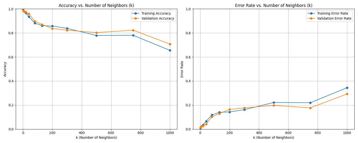
Fig. 13.2 Case_2_train_val.png

Table 13.4 Deliverables

Deliverables	Description
tp3_team_1_teamnumber.pdf	Flowchart(s) for this task.
tp3_team_1_teamnumber.py	Your completed Python code.