Dec 04, 2025 | 1804 words | 18 min read
13.1.3. Task 3#
Learning Objectives#
Understand the concept of binary logistic regression for classification.
Implement the sigmoid function and logistic regression prediction.
Train the model using gradient descent to minimize binary cross-entropy loss.
Evaluate performance using accuracy and error rate on train/val/test sets.
Task Instructions#
In this task, you will build and train a binary logistic regression model from scratch using NumPy to classify traffic signs as either:
Stop sign (label = 1)
Right turn sign (label = 0)
The model will use features extracted earlier (e.g., hue mean, hue standard deviation, big circle presence, number of lines, etc.).
Note
For the functions described below, the order of arguments and outputs matters. Please ask TAs for guidance and explanation.
1. Concept Recap - What is Logistic Regression?#
Think of logistic regression as a way to make “yes/no” decisions based on multiple pieces of information. Instead of giving you a simple yes or no, it gives you a probability (a number between 0 and 1) that represents how confident it is about the answer.
How It Works Step-by-Step#
Step 1: Combine All Features (The Linear Part)#
First, we take all the features and combine them using weights (like importance scores):
\( z = w_1 \times \text{feature}_1 + w_2 \times \text{feature}_2 + ... + w_n \times \text{feature}_n + b \)
Breaking this down:
Each feature gets multiplied by a weight (w₁, w₂, etc.)
The weights tell us how important each feature is
We add a “bias” term (b) at the end
The result (z) can be any number (positive, negative, or zero)
Example with traffic signs: If we have features like:
Hue mean = 0.6
Number of lines = 8
Big circle present = 1 (yes)
And weights like:
w₁ = 2.5 (hue is very important)
w₂ = 0.8 (lines matter somewhat)
w₃ = 1.2 (circle presence is important)
b = -1.0 (overall bias)
Then: z = 2.5×0.6 + 0.8×8 + 1.2×1 + (-1.0) = 1.5 + 6.4 + 1.2 - 1.0 = 8.1
Step 2: Convert to Probability (The Sigmoid Function)#
The problem is that z can be any number, but we want a probability between 0 and 1. This is where the sigmoid function comes in:
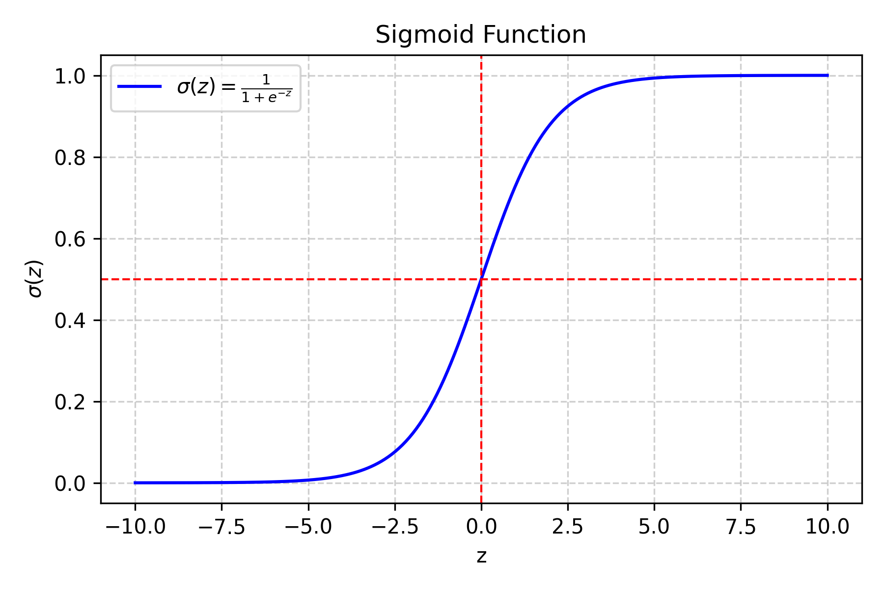
Fig. 13.7 Sigmoid function#
What does this do?
If z is very large and positive → σ(z) gets close to 1 (100% probability)
If z is very large and negative → σ(z) gets close to 0 (0% probability)
If z = 0 → σ(z) = 0.5 (50% probability)
Why the sigmoid function?
It’s smooth and differentiable (important for training)
It naturally maps any number to [0,1]
It has a nice S-shape that makes sense for probabilities
Example:
If z = 8.1 (from our traffic sign example):
σ(8.1) = 1/(1 + e^(-8.1)) = 1/(1 + 0.0003) ≈ 0.9997
This means 99.97% chance it’s a stop sign!
Step 3: Make the Final Decision#
If σ(z) ≥ 0.5 → predict class 1 (stop sign)
If σ(z) < 0.5 → predict class 0 (right turn sign)
2. Understanding the Loss Function#
Why Do We Need a Loss Function?#
The loss function tells us how “wrong” our predictions are. We want to minimize this to make our model better.
Binary Cross-Entropy Loss Explained#
For a Single Example:#
The loss depends on the true label (y) and our predicted probability (ŷ):
Case 1: True label is 1 (stop sign)
If we predict ŷ = 0.9 (90% confident it’s a stop sign) → Low loss
If we predict ŷ = 0.1 (10% confident it’s a stop sign) → High loss
Case 2: True label is 0 (right turn sign)
If we predict ŷ = 0.1 (10% confident it’s a stop sign) → Low loss
If we predict ŷ = 0.9 (90% confident it’s a stop sign) → High loss
Mathematical Formula:#
\( \text{loss} = \begin{cases} -\log(\hat{y}) & \text{if } y = 1 \\ -\log(1 - \hat{y}) & \text{if } y = 0 \end{cases} \)
Why the negative log?
When ŷ is close to 1 and y = 1, log(ŷ) is close to 0, so -log(ŷ) is close to 0 (low loss)
When ŷ is close to 0 and y = 1, log(ŷ) is very negative, so -log(ŷ) is very large (high loss)
The negative sign ensures that better predictions give lower loss values
Average Loss for All Examples:#
\( J(w,b) = -\frac{1}{m} \sum_{i=1}^m \left[ y^{(i)} \log(\hat{y}^{(i)}) + (1 - y^{(i)}) \log(1 - \hat{y}^{(i)}) \right] \)
Breaking this down:
m = number of examples
For each example i:
If y⁽ⁱ⁾ = 1: add log(ŷ⁽ⁱ⁾)
If y⁽ⁱ⁾ = 0: add log(1 - ŷ⁽ⁱ⁾)
Take the negative of the average
This gives us one number representing how well our model is doing
Note
The binary cross-entropy loss is also called “log loss” and is the standard loss function for binary classification problems. It heavily penalizes confident wrong predictions.
3. Training with Gradient Descent - Step by Step#
What is Gradient Descent?#
Imagine you’re on a hill and want to get to the bottom. You look around to see which direction is downhill, take a step in that direction, and repeat. Gradient descent works the same way - it finds the direction that makes the loss smaller and moves in that direction.
The Training Process:#
Step 1: Initialize Parameters#
Weights (w): Start with small random numbers (like between -0.1 and 0.1)
Why random? If we start with all zeros, all features would have the same importance
Why small? Large initial values can make training unstable
Bias (b): Start with 0
This represents the overall tendency to predict one class over the other
Step 2: The Training Loop#
Repeat these steps many times:
A. Make Predictions
Use current w and b to predict ŷ for all examples
ŷ = σ(w·x + b) for each example
B. Calculate Loss
Use the binary cross-entropy formula from above
This tells us how well we’re doing
C. Calculate Gradients (The “Downhill Direction”) The gradient tells us how much the loss changes when we change each parameter:
\( \frac{\partial J}{\partial w} = \frac{1}{m} X^T (\hat{y} - y) \)
\( \frac{\partial J}{\partial b} = \frac{1}{m} \sum_{i=1}^m (\hat{y}^{(i)} - y^{(i)}) \)
What do these mean?
∂J/∂w: How much the loss changes when we change the weights
∂J/∂b: How much the loss changes when we change the bias
(ŷ - y): The prediction error for each example
X^T: The transpose of our feature matrix (this is just matrix math)
D. Update Parameters Move in the direction that reduces the loss:
\( w := w - \alpha \frac{\partial J}{\partial w} \)
\( b := b - \alpha \frac{\partial J}{\partial b} \)
What is α (alpha)?
This is the learning rate - how big of a step we take
Typical values: 0.01, 0.1, or 0.001
Step 3: When to Stop#
Maximum iterations reached: We’ve tried enough times
Loss change is tiny: We’re not improving much anymore
Loss is very small: We’re doing well enough
Warning
Be careful with the learning rate! If it’s too high, your loss might oscillate or even increase. If it’s too low, training will be very slow. Start with 0.01 and adjust based on how the loss behaves.
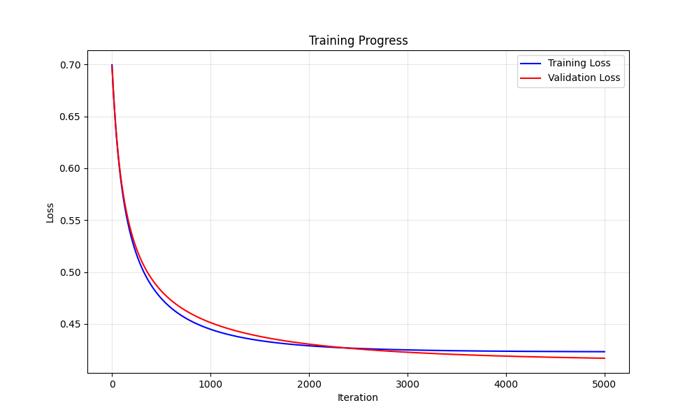
Fig. 13.8 Training loss#
4. Evaluation Metrics - How Good is Our Model?#
Accuracy#
\( \text{Accuracy} = \frac{\text{Number of correct predictions}}{\text{Total number of examples}} \)
What’s a good accuracy?
Random guessing: 50% (for binary classification)
Good model: 80%+
Excellent model: 90%+
Error Rate#
\( \text{Error Rate} = 1 - \text{Accuracy} \)
Why Both Metrics?#
Accuracy tells us what we’re doing right
Error rate tells us what we’re doing wrong
Sometimes one is more intuitive than the other
5. Functions to Implement - Detailed Breakdown#
Function 1: calculate_sigmoid(z)#
Purpose: Convert any number to a probability between 0 and 1
Input: z (any number) Output: probability between 0 and 1
Formula: \(σ(z) = \frac{1}{(1 + e^{-z})})\)
Hint
Use
np.exp()for \(e^z\)Be careful with very large negative z values (can cause overflow, consider using
np.clip())Consider adding a small epsilon (like 1e-15) to avoid division by zero
Function 2: predict_proba(X, w, b)#
Purpose: Get probabilities for all examples in a dataset
Inputs:
X: feature matrix (shape: m × n where m = examples, n = features)
w: weight vector (shape: n × 1)
b: bias (scalar)
Output: probability array (shape: m × 1)
Steps:
Calculate z = X·w + b (matrix multiplication)
Apply sigmoid to each z value
Return the probabilities
Implementation hints:
Use
np.dot()or@operator for matrix multiplicationMake sure dimensions match: X is (m,n), w is (n,1), result is (m,1)
You can use broadcasting: X @ w + b will work if b is a scalar
Function 3: predict_labels(X, w, b, threshold=0.5)#
Purpose: Convert probabilities to class labels (0 or 1)
Inputs: Same as predict_proba, plus threshold (default 0.5) Output: array of 0s and 1s
Steps:
Get probabilities using predict_proba
Compare each probability to threshold
Return 1 if ≥ threshold, 0 otherwise
Implementation hints:
Use
>=comparison operatorConvert boolean array to integers with
.astype(int)The threshold parameter lets you adjust the decision boundary
Function 4: compute_loss_and_grads(X, y, w, b)#
Purpose: Calculate loss and gradients for current parameters
Inputs:
X: feature matrix
y: true labels (0s and 1s)
w: current weights
b: current bias
Outputs:
loss: scalar value
dw: gradient with respect to w
db: gradient with respect to b
Steps:
Get predictions using predict_proba
Calculate loss using binary cross-entropy formula
Calculate gradients using the formulas from section 3
Return all three values
Implementation hints:
Be careful with log(0) - add small epsilon to predictions
Use
np.sum()for the bias gradientUse
X.T @ (y_pred - y)for the weight gradient
Function 5: train_logistic_regression(...)#
Purpose: Train the model using gradient descent
Inputs:
X_train, y_train: training data
learning_rate: step size for gradient descent
num_iterations: how many times to update parameters
(optional) X_val, y_val: validation data for monitoring
Outputs:
w_final, b_final: trained parameters
loss_history: list of loss values during training
Steps:
Initialize w and b
For each iteration:
Compute loss and gradients
Update parameters
Store loss value
(optional) Check validation performance
Return final parameters and loss history
Implementation hints:
Start with small random weights:
np.random.randn(n_features) * 0.01Store loss after each iteration to monitor progress
Consider early stopping if validation loss increases
Function 6: calculate_metrics(predicted_labels, true_labels)#
Purpose: Calculate accuracy and error rate
Inputs:
predicted_labels: array of 0s and 1s from your model
true_labels: array of actual 0s and 1s
Outputs:
accuracy: percentage of correct predictions
error_rate: percentage of incorrect predictions
Implementation hints:
Use
np.mean(predicted_labels == true_labels)for accuracyOr count manually:
np.sum(predicted_labels == true_labels) / len(true_labels)Error rate is just 1 - accuracy
Function 7: evaluate_logistic_regression(...)#
Purpose: Evaluate the trained model on any dataset
Inputs:
X, y: data to evaluate on
w, b: trained parameters
Outputs:
accuracy, error_rate: performance metrics
Steps:
Use predict_labels to get predictions
Use calculate_metrics to get performance
Return the results
6. Implementation Notes and Best Practices#
Data Preprocessing - Feature Standardization#
Why standardize?
Features might have very different scales (e.g., hue 0-1, number of lines 0-20)
This can make training unstable
Standardization puts all features on the same scale
How to do it:
Calculate mean and standard deviation of each feature using training data only
For each feature: (value - mean) / standard_deviation
Apply the same transformation to validation and test data
Example:
# Calculate statistics from training data
feature_means = np.mean(X_train, axis=0)
feature_stds = np.std(X_train, axis=0)

# Standardize training data
X_train_std = (X_train - feature_means) / feature_stds

# Apply same transformation to validation/test data
X_val_std = (X_val - feature_means) / feature_stds
X_test_std = (X_test - feature_means) / feature_stds
Important
Always calculate standardization statistics (mean and std) from the training data only, then apply those same values to validation and test data. This prevents data leakage!
Hyperparameter Tuning#
Learning rate (α):
Start with 0.01 or 0.1
If loss oscillates wildly → decrease learning rate
If loss decreases very slowly → increase learning rate
Number of iterations:
Start with 1000-5000
Monitor loss - if it’s still decreasing, increase iterations
If loss plateaus early, you can stop earlier
Initial weights:
Small random values (multiply by 0.01 or 0.001)
Avoid all zeros (all features would start with equal importance)
Monitoring Training Progress#
What to watch for:
Loss should decrease over time
If loss increases → learning rate too high
If loss plateaus → might need more iterations or different learning rate
If loss oscillates → learning rate too high
Common Pitfalls and Solutions#
Problem: Loss becomes NaN (Not a Number) Solution:
Check for division by zero in sigmoid
Add small epsilon to log calculations
Reduce learning rate
Problem: Model always predicts the same class Solution:
Check if your data is balanced
Verify feature standardization
Try different initial weights
Problem: Training is very slow Solution:
Increase learning rate (carefully)
Check if features are properly scaled
Reduce number of features if possible
Warning
If your loss becomes NaN or infinity, immediately check your sigmoid function and gradient calculations. This usually indicates a numerical overflow or division by zero.
7. Complete Implementation Example Structure#
Here’s how your main training function might look:
def train_logistic_regression(X_train, y_train, X_val=None, y_val=None,
                            learning_rate=0.01, num_iterations=1000):
    """
    Train logistic regression model using gradient descent

    Parameters:
    - X_train, y_train: training data
    - X_val, y_val: validation data (optional)
    - learning_rate: step size for gradient descent
    - num_iterations: number of training iterations

    Returns:
    - w_final, b_final: trained parameters
    - loss_history: list of loss values during training
    """

    # Get dimensions
    m, n = X_train.shape

    # Initialize parameters
    w = np.random.randn(n) * 0.01
    b = 0.0

    # Store loss history
    loss_history = []

    # Training loop
    for i in range(num_iterations):
        # Forward pass: compute loss and gradients
        loss, dw, db = compute_loss_and_grads(X_train, y_train, w, b)

        # Update parameters
        w = w - learning_rate * dw
        b = b - learning_rate * db

        # Store loss
        loss_history.append(loss)

        # Optional: print progress every 100 iterations
        if i % 100 == 0:
            print(f"Iteration {i}, Loss: {loss:.4f}")

    return w, b, loss_history
8. Testing Your Implementation#
Simple Test Cases#
Sigmoid function:
sigmoid(0) should equal 0.5
sigmoid(very large positive) should be close to 1
sigmoid(very large negative) should be close to 0
Predictions:
With all-zero weights and bias, all predictions should be 0.5
With very large positive weights, predictions should be close to 1
Loss calculation:
Perfect predictions should give loss close to 0
Random predictions should give loss around 0.69
Sanity Checks#
Loss should decrease during training
Final accuracy should be better than random guessing (50%)
Weights should not be all zero after training
Deliverables#
Code: A Python file implementing binary logistic regression from scratch.
Report section:
Briefly explain how logistic regression works.
Describe the loss function.
Document your training procedure and chosen hyperparameters.
Report accuracy and error rate for train/val/test sets.
Deliverables |
Description |
|---|---|
tp3_team_3_teamnumber.pdf |
Flowchart(s) for this task. |
tp3_team_3_teamnumber.py |
Your completed Python code. |