\[ \begin{align}\begin{aligned}\newcommand\blank{~\underline{\hspace{1.2cm}}~}\\% Bold symbols (vectors) \newcommand\bs[1]{\mathbf{#1}}\\% Differential \newcommand\dd[2][]{\mathrm{d}^{#1}{#2}} % use as \dd, \dd{x}, or \dd[2]{x}\\% Poor man's siunitx \newcommand\unit[1]{\mathrm{#1}} \newcommand\num[1]{#1} \newcommand\qty[2]{#1~\unit{#2}}\\\newcommand\per{/} \newcommand\squared{{}^2} \newcommand\cubed{{}^3} % % Scale \newcommand\milli{\unit{m}} \newcommand\centi{\unit{c}} \newcommand\kilo{\unit{k}} \newcommand\mega{\unit{M}} % % Percent \newcommand\percent{\unit{{\kern-4mu}\%}} % % Angle \newcommand\radian{\unit{rad}} \newcommand\degree{\unit{{\kern-4mu}^\circ}} % % Time \newcommand\second{\unit{s}} \newcommand\s{\second} \newcommand\minute{\unit{min}} \newcommand\hour{\unit{h}} % % Distance \newcommand\meter{\unit{m}} \newcommand\m{\meter} \newcommand\inch{\unit{in}} \newcommand\foot{\unit{ft}} % % Force \newcommand\newton{\unit{N}} \newcommand\kip{\unit{kip}} % kilopound in "freedom" units - edit made by Sri % % Mass \newcommand\gram{\unit{g}} \newcommand\g{\gram} \newcommand\kilogram{\unit{kg}} \newcommand\kg{\kilogram} \newcommand\grain{\unit{grain}} \newcommand\ounce{\unit{oz}} % % Temperature \newcommand\kelvin{\unit{K}} \newcommand\K{\kelvin} \newcommand\celsius{\unit{{}^\circ C}} \newcommand\C{\celsius} \newcommand\fahrenheit{\unit{{}^\circ F}} \newcommand\F{\fahrenheit} % % Area \newcommand\sqft{\unit{sq\,\foot}} % square foot % % Volume \newcommand\liter{\unit{L}} \newcommand\gallon{\unit{gal}} % % Frequency \newcommand\hertz{\unit{Hz}} \newcommand\rpm{\unit{rpm}} % % Voltage \newcommand\volt{\unit{V}} \newcommand\V{\volt} \newcommand\millivolt{\milli\volt} \newcommand\mV{\milli\volt} \newcommand\kilovolt{\kilo\volt} \newcommand\kV{\kilo\volt} % % Current \newcommand\ampere{\unit{A}} \newcommand\A{\ampere} \newcommand\milliampereA{\milli\ampere} \newcommand\mA{\milli\ampere} \newcommand\kiloampereA{\kilo\ampere} \newcommand\kA{\kilo\ampere} % % Resistance \newcommand\ohm{\Omega} \newcommand\milliohm{\milli\ohm} \newcommand\kiloohm{\kilo\ohm} % correct SI spelling \newcommand\kilohm{\kilo\ohm} % "American" spelling used in siunitx \newcommand\megaohm{\mega\ohm} % correct SI spelling \newcommand\megohm{\mega\ohm} % "American" spelling used in siunitx % % Capacitance \newcommand\farad{\unit{F}} \newcommand\F{\farad} \newcommand\microfarad{\micro\farad} \newcommand\muF{\micro\farad} % % Inductance \newcommand\henry{\unit{H}} \newcommand\H{\henry} \newcommand\millihenry{\milli\henry} \newcommand\mH{\milli\henry} % % Power \newcommand\watt{\unit{W}} \newcommand\W{\watt} \newcommand\milliwatt{\milli\watt} \newcommand\mW{\milli\watt} \newcommand\kilowatt{\kilo\watt} \newcommand\kW{\kilo\watt} % % Energy \newcommand\joule{\unit{J}} \newcommand\J{\joule} % % Composite units % % Torque \newcommand\ozin{\unit{\ounce}\,\unit{in}} \newcommand\newtonmeter{\unit{\newton\,\meter}} % % Pressure \newcommand\psf{\unit{psf}} % pounds per square foot \newcommand\pcf{\unit{pcf}} % pounds per cubic foot \newcommand\pascal{\unit{Pa}} \newcommand\Pa{\pascal} \newcommand\ksi{\unit{ksi}} % kilopound per square inch \newcommand\bar{\unit{bar}} \end{aligned}\end{align} \]

Dec 04, 2025 | 1480 words | 15 min read

12.2.1. Task 1

Learning Objectives

• Understand the concepts of kernel filtering

• Implement a Gaussian filter from scratch

Task Instructions

Save the flowcharts for this task in tp2_team_1_teamnumber.pdf You will also need to include these flowcharts in your final report.

In this part of the task, you will write a function called gaussian_filter to blur a grayscale image. Name your program file as specified in tp2_team_1_teamnumber.py.

Why are we blurring an image?

In order to classify these images, it will be helpful to extract features like whether a circle is in the image or how many lines are in the image. In order to do this we need to isolate the edges of the objects in the image (we will go into more depth about edge detection in the next task Section 12.2.2).

While it might seem counterintuitive at first, blurring a grayscale image is an important step before being able to perform operations like edge detection. The blurring helps to remove minor details like texture, while retaining the more major details like edges. This is something that is very noticeable when squinting your eyes while looking at an object, you lose a lot of the minor details of the object, but the overall edges of the object remain.

Note

For easier viewing, we recommend using light mode for the following figures.

Why Gaussian?

One method of blurring an image is to go through an image, pixel by pixel, and reassign each pixel’s value to be the average of all the neighboring pixels’ values. This method does blur the image and is simple to implement, but fails to preserve enough detail to be very useful in our case. Let’s see the difference between what a “mean blur” and a “Gaussian blur” might be :

Let’s start with the following 5x5 image :

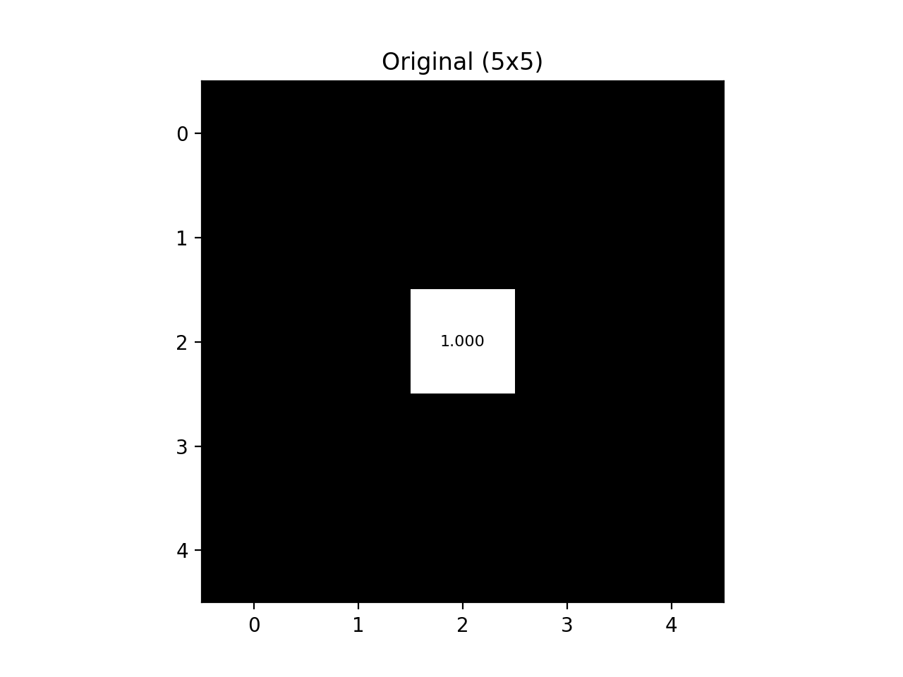
Fig. 12.1 Original Black-White Grid

Each of the pixels in this image are labeled with their respective grayscale value [0,1].

We will now go through the image, pixel by pixel, reassigning each pixel to be the average value of itself and all adjacent pixels. On a 2D grid like this, the adjacent pixels for any given pixel are the pixels located in a \(3\times3\) grid centered at that pixel. This “neighborhood” is known as the kernel. For example, the pixel in (0,0) will be equal to the average of (0,0), (0,1), (1,0), and (1,1) in the new image (which is still 0). The output would look like this :

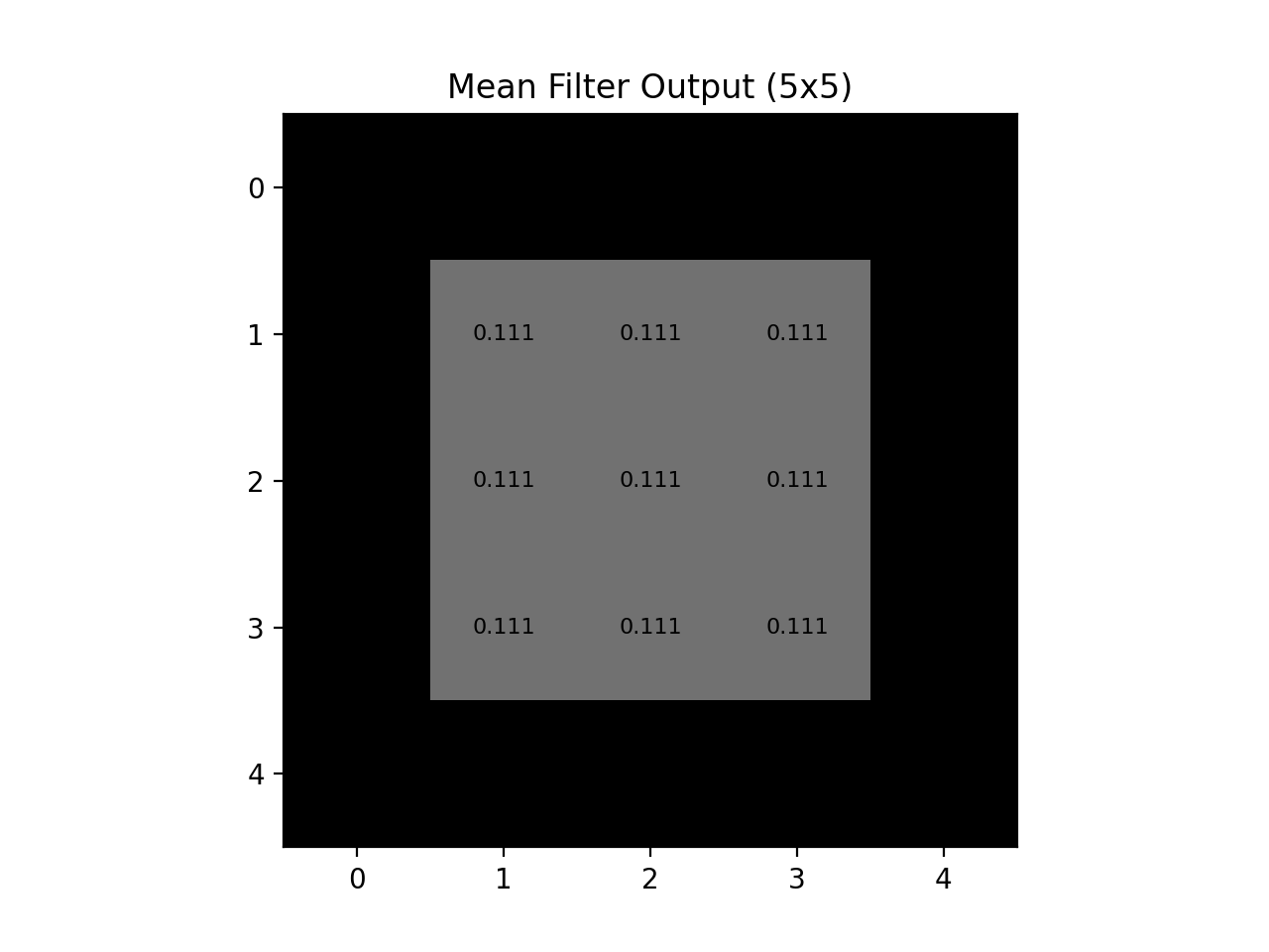
Fig. 12.2 Mean Blur Output

As we can see, the “mean blur” gives equal weight to all pixels in the kernel and this results in a blocky blurred image. The Gaussian filter gives varying weights to the pixels in the kernel, with pixels farther away from the center pixel having exponentially less weight than the pixels nearest to the center. With the same size kernel (\(3\times3\)) the Gaussian blur outputs the following :

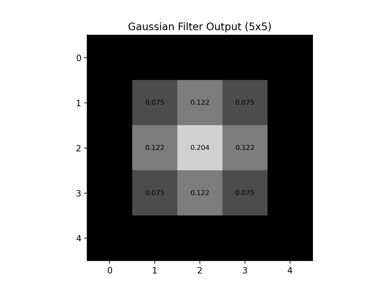
Fig. 12.3 Gaussian Blur Output

Even with an image as small as this, the Gaussian blur retains far more similarity to the original image. The power of the Gaussian filter is even more pronounced in a larger image, so let’s see that with an \(11\times11\) sized image and a \(5\times5\) kernel :

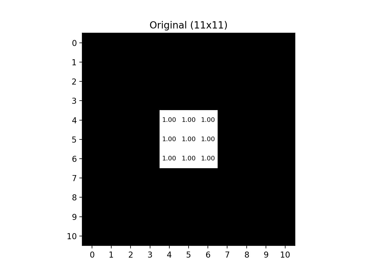
Fig. 12.4 Large Black-White Grid ``

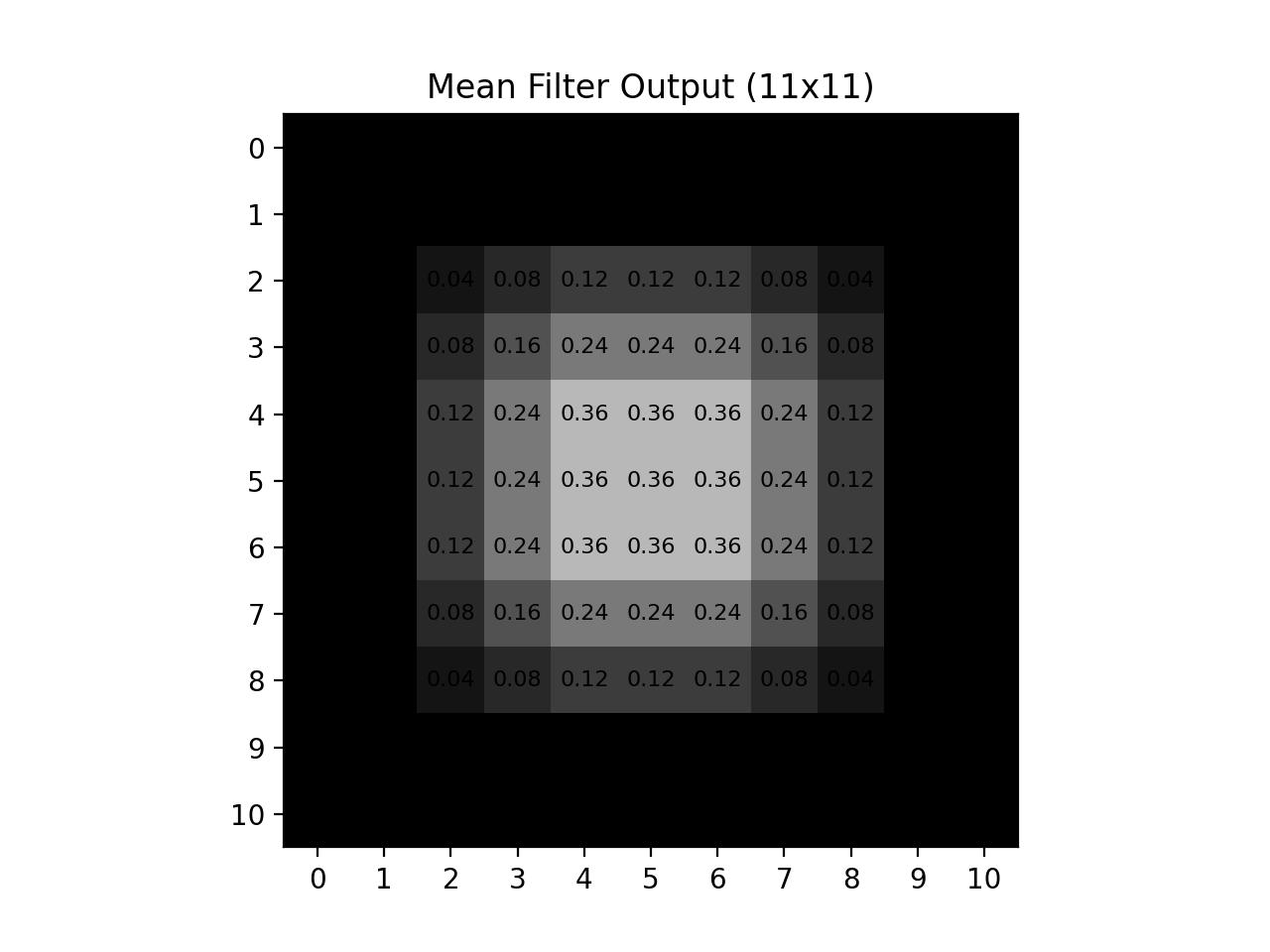
Fig. 12.5 Large Mean Blur Output

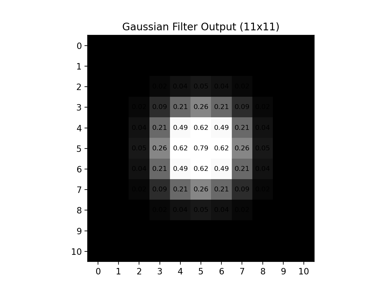
Fig. 12.6 Large Gaussian Blur Output

How do we construct the Gaussian filter?

The 2D Gaussian function is the function that gives the relative weights of the pixels in the kernel. The function is defined as :

\[ G(x, y) = \frac{1}{2\pi\sigma^2}\cdot e^{\left(-\frac{x^2 + y^2}{2\sigma^2}\right)} \]

where:

• \(G(x, y)\) is the weight of the pixel at the relative position \((x, y)\),

• \(x\) and \(y\) are the distances from the reference pixel. In a \(3\times3\) kernel \((x,y)\) will be all the pair combinations of the numbers in \([-2,-1,0,1,2]\).

• \(\sigma\) is the standard deviation and controls the “spread” of the blur. By default, \(\sigma\) will be 1.

Note

Feel free to experiment with other values of \(\sigma\). However, your submission should use \(\sigma = 1\).

How do we choose the size of the kernel?

The size of the kernel should be chosen so that the pixels farthest from the center (for a \(7\times7\) kernel that’s the pixels \(-3\) and \(+3\) from the center) return a value as close to zero as possible from \(G(x,y)\) without actually being zero (this would be a waste of computation).

This sounds like a difficult problem to solve, so let’s simplify the 2D Gaussian function to just a 1 dimensional slice down the center :

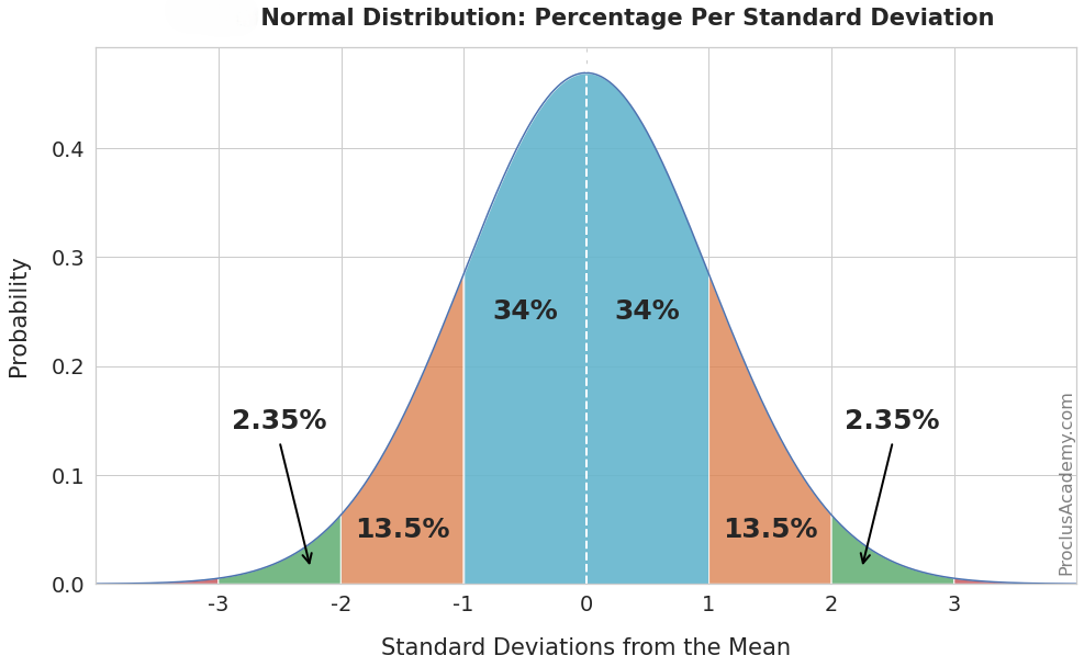
Fig. 12.7 Normal Curve

From this view, we can see that values \(-4\) and \(+4\) standard deviations (\(\sigma\)) away from the mean are essentially zero (in other words they would have negligible influence on the center pixel), so we will use pixels within \(-3\) and \(+3\) standard deviations from the center. Under this rule we cover about 99.7% of the possible values that the 1D Gaussian function can output, which means that we are maximizing the number of pixels that have influence on a given pixel without wasting computations on those pixels that are too far away. Since the 2D Gaussian function follows this shape in both \(x\) and \(y\) directions, the rule still applies for the 2D function.

To determine the size of your kernel, we use the following equation :

\[ \text{kernel}\_ \text{size} = 2 \times 3\sigma + 1 \]

• This uses our \(3\sigma\) rule (\(3\sigma\) to the right and left of the center pixel)

• Then we add \(1\) to account for the center pixel itself

• If we say \(\sigma = 1\), then we get \(\text{kernel}\_ \text{size} = 7\), so we say our kernel has a size of \(7\times7\)

Note

The only constraint on \(\sigma\) is that \(\sigma > 0\).

To ensure that the kernel size is an odd number, you should round up the value of 3 * sigma.

What happens at the edges?

You may have already asked how we handle pixels at the edges of an image, as these pixels don’t have a full kernel worth of neighbors. To fix this issue we simply pad the image according to how large our kernel is. This ensures that ALL pixels in the original image have a full kernel and that the filter won’t run into any strange cases where a pixel does not exist. For simplicity, we will be padding with zeros like was done in Section 11.2.2, but using the following formula to determine how much to pad our image :

\[ \text{pad}\_ \text{size} = \frac{\text{kernel}\_ \text{size} - 1}{2} \]

Note

Depending on your workflow, you may find it easier to use the np.pad() function to pad the image. See Section 12.1.1 for details.

Putting it all together

You will now write a function gaussian_filter that takes in a grayscale image and \(\sigma\) as parameters and outputs a uint8 NumPy array of the Gaussian blurred image. You should first convert the original image using the rgb_to_grayscale function from Section 11.2.1 before passing it into this new function.

The function will need to :

1. Determine the kernel size

2. Initialize the kernel using \(G(x,y)\) and the values of \(x\) and \(y\) in your kernel’s range and normalize the kernel by dividing each of these values by the sum of all the values in the kernel (this ensures the output pixel value is within [0,1]).

3. Initialize an output array that is the same size as the input image (you will convert this array to an image as your return output)

4. Create a padded image based on the kernel size (padding with zeros).

5. Iterate through each pixel of the output image. For each pixel in the output image you need to :

• create an array of all the pixels in the kernel using the padded image

• multiply the group of pixels by the weights in the kernel

• assign the sum of these products to be the output pixel’s value.

Example:

Let’s say \(\sigma=1\) and the image we are using is Original Black-White Grid.

1. The size of our kernel is \(7\times7\) using our formula, but in this example we will be using a \(3\times3\) kernel for readability.

2. The kernel would be:

\[\begin{split} \underbrace{ \begin{array}{|c|c|c|c|c|} \hline G(-1,1)&G(0,1)&G(1,1)\\ \hline G(-1,0)&G(0,0)&G(1,0)\\ \hline G(-1,-1)&G(0,-1)&G(1,-1)\\ \hline \end{array}}_{\text{Function Values}}~\approx ~ \underbrace{ \begin{array}{|c|c|c|c|c|} \hline 0.06&0.10&0.06\\ \hline 0.10&0.16&0.10\\ \hline 0.06&0.10&0.06\\ \hline \end{array}}_{\text{Decimal Values}} ~\Rightarrow ~ \underbrace{ \begin{array}{|c|c|c|} \hline 0.075&0.125&0.075\\ \hline 0.125&0.20&0.125\\ \hline 0.075&0.125&0.075\\ \hline \end{array}}_{\text{Normalize (divide by sum of decimal values)}} \end{split}\]

3. The original image is a \(5\times5\) grid represented by :

\[\begin{split} \begin{matrix} 0&0&0&0&0\\ 0&0&0&0&0\\ 0&0&1&0&0\\ 0&0&0&0&0\\ 0&0&0&0&0\\ \end{matrix} \end{split}\]

So the initialized output is represented as :

\[\begin{split} \begin{matrix} 0&0&0&0&0\\ 0&0&0&0&0\\ 0&0&0&0&0\\ 0&0&0&0&0\\ 0&0&0&0&0\\ \end{matrix} \end{split}\]

4. The pad size we will use is \(1\) (using the formula, based on our \(3\times3\) example size), so our new padded image will be a \(7\times7\) grid represented by :

\[\begin{split} \begin{matrix} 0&0&0&0&0&0&0\\ 0&\textcolor{red}{0}&\textcolor{red}{0}&\textcolor{red}{0}&\textcolor{red}{0}&\textcolor{red}{0}&0\\ 0&\textcolor{red}{0}&\textcolor{red}{0}&\textcolor{red}{0}&\textcolor{red}{0}&\textcolor{red}{0}&0\\ 0&\textcolor{red}{0}&\textcolor{red}{0}&\textcolor{red}{1}&\textcolor{red}{0}&\textcolor{red}{0}&0\\ 0&\textcolor{red}{0}&\textcolor{red}{0}&\textcolor{red}{0}&\textcolor{red}{0}&\textcolor{red}{0}&0\\ 0&\textcolor{red}{0}&\textcolor{red}{0}&\textcolor{red}{0}&\textcolor{red}{0}&\textcolor{red}{0}&0\\ 0&0&0&0&0&0&0\\ \end{matrix} \end{split}\]

5. We will begin iterating through the pixels starting at the green value :

\[\begin{split} \begin{matrix} 0&0&0&0&0&0&0\\ 0&\textcolor{green}{0}&\textcolor{red}{0}&\textcolor{red}{0}&\textcolor{red}{0}&\textcolor{red}{0}&0\\ 0&\textcolor{red}{0}&\textcolor{red}{0}&\textcolor{red}{0}&\textcolor{red}{0}&\textcolor{red}{0}&0\\ 0&\textcolor{red}{0}&\textcolor{red}{0}&\textcolor{red}{1}&\textcolor{red}{0}&\textcolor{red}{0}&0\\ 0&\textcolor{red}{0}&\textcolor{red}{0}&\textcolor{red}{0}&\textcolor{red}{0}&\textcolor{red}{0}&0\\ 0&\textcolor{red}{0}&\textcolor{red}{0}&\textcolor{red}{0}&\textcolor{red}{0}&\textcolor{red}{0}&0\\ 0&0&0&0&0&0&0\\ \end{matrix} \end{split}\]

Take the pixels within the kernel (in magenta), multiply that with the kernel and find the sum of the resulting array of products :

\[\begin{split} \begin{matrix} 0&0&0&0&0&0&0\\ 0&\textcolor{green}{0}&\textcolor{red}{0}&\textcolor{red}{0}&\textcolor{red}{0}&\textcolor{red}{0}&0\\ 0&\textcolor{red}{0}&\textcolor{red}{0}&\textcolor{red}{0}&\textcolor{red}{0}&\textcolor{red}{0}&0\\ 0&\textcolor{red}{0}&\textcolor{red}{0}&\textcolor{red}{1}&\textcolor{red}{0}&\textcolor{red}{0}&0\\ 0&\textcolor{red}{0}&\textcolor{red}{0}&\textcolor{red}{0}&\textcolor{red}{0}&\textcolor{red}{0}&0\\ 0&\textcolor{red}{0}&\textcolor{red}{0}&\textcolor{red}{0}&\textcolor{red}{0}&\textcolor{red}{0}&0\\ 0&0&0&0&0&0&0\\ \end{matrix} ~ \Rightarrow~ \begin{matrix} \textcolor{magenta}{0}&\textcolor{magenta}{0}&\textcolor{magenta}{0}&0&0&0&0\\ \textcolor{magenta}{0}&\textcolor{magenta}{0}&\textcolor{magenta}{0}&\textcolor{red}{0}&\textcolor{red}{0}&\textcolor{red}{0}&0\\ \textcolor{magenta}{0}&\textcolor{magenta}{0}&\textcolor{magenta}{0}&\textcolor{red}{0}&\textcolor{red}{0}&\textcolor{red}{0}&0\\ 0&\textcolor{red}{0}&\textcolor{red}{0}&\textcolor{red}{1}&\textcolor{red}{0}&\textcolor{red}{0}&0\\ 0&\textcolor{red}{0}&\textcolor{red}{0}&\textcolor{red}{0}&\textcolor{red}{0}&\textcolor{red}{0}&0\\ 0&\textcolor{red}{0}&\textcolor{red}{0}&\textcolor{red}{0}&\textcolor{red}{0}&\textcolor{red}{0}&0\\ 0&0&0&0&0&0&0\\ \end{matrix} \end{split}\]

\[\begin{split} \text{Pixels in Kernel} =~ \begin{matrix} \textcolor{magenta}{0_1}&\textcolor{magenta}{0_2}&\textcolor{magenta}{0_3}\\ \textcolor{magenta}{0_4}&\textcolor{magenta}{0_5}&\textcolor{magenta}{0_6}\\ \textcolor{magenta}{0_7}&\textcolor{magenta}{0_8}&\textcolor{magenta}{0_9} \end{matrix} \Rightarrow P = [\textcolor{magenta}{0_1},\textcolor{magenta}{0_2},\textcolor{magenta}{0_3},\textcolor{magenta}{0_4},\textcolor{magenta}{0_5},\textcolor{magenta}{0_6},\textcolor{magenta}{0_7},\textcolor{magenta}{0_8},\textcolor{magenta}{0_9}] \end{split}\]

\[\begin{split} \text{Kernel} = ~ \begin{array}{|c|c|c|} \hline 0.075&0.125&0.075\\ \hline 0.125&0.20&0.125\\ \hline 0.075&0.125&0.075\\ \hline \end{array} \Rightarrow K \end{split}\]

\[ K = [0.075,~0.125,~0.075,~0.125,~0.20,~0.125,~0.075,~0.125,~0.075] \]

\[ P\cdot K = [\textcolor{magenta}{0},\textcolor{magenta}{0},\textcolor{magenta}{0},\textcolor{magenta}{0},\textcolor{magenta}{0},\textcolor{magenta}{0},\textcolor{magenta}{0},\textcolor{magenta}{0},\textcolor{magenta}{0}]\cdot [0.075,~0.125,~0.075,~0.125,~0.20,~0.125,~0.075,~0.125,~0.075] \]

\[ =[0,0,0,0,0,0,0,0,0] \Rightarrow \text{Sum}(P\cdot K) = 0 \]

Referencing the same pixel in the output, we assign the value to the sum of \(P\cdot K\) :

\[\begin{split} \begin{matrix} \textcolor{green}{0}&0&0&0&0\\ 0&0&0&0&0\\ 0&0&0&0&0\\ 0&0&0&0&0\\ 0&0&0&0&0\\ \end{matrix}\Rightarrow \textcolor{green}{0} = 0 \end{split}\]

We then iterate to the next pixel and repeat the steps :

\[\begin{split} \begin{matrix} 0&0&0&0&0&0&0\\ 0&\textcolor{red}{0}&\textcolor{green}{0}&\textcolor{red}{0}&\textcolor{red}{0}&\textcolor{red}{0}&0\\ 0&\textcolor{red}{0}&\textcolor{red}{0}&\textcolor{red}{0}&\textcolor{red}{0}&\textcolor{red}{0}&0\\ 0&\textcolor{red}{0}&\textcolor{red}{0}&\textcolor{red}{1}&\textcolor{red}{0}&\textcolor{red}{0}&0\\ 0&\textcolor{red}{0}&\textcolor{red}{0}&\textcolor{red}{0}&\textcolor{red}{0}&\textcolor{red}{0}&0\\ 0&\textcolor{red}{0}&\textcolor{red}{0}&\textcolor{red}{0}&\textcolor{red}{0}&\textcolor{red}{0}&0\\ 0&0&0&0&0&0&0\\ \end{matrix} \end{split}\]

Note

You will not be changing values in the input image or the padded image, ONLY in the output image.

Main method

Your main method will ask the user for an image file path, then use the load_img function from Section 11.2.1 to load the image into an array. Next, use the rgb_to_grayscale function from Section 11.2.1 to convert it to grayscale. Then, call your gaussian_filter function to blur the image. Finally, display the image to the user. See the examples provided below.

Organize your code to use functions that break up the task into manageable pieces. Use the files provided in the Table 12.3 to test your code.

Table 12.3 Image Files

Image File Name	Description
ref_col.png	A color image
ref_col_b.png	A color image

Sample Output

Use the values in Table 12.4 below to test your program.

Table 12.4 Test Cases

Case	image_path
1	ref_col.png
2	ref_col_b.png

Ensure your program’s output matches the provided samples exactly. This includes all characters, white space, and punctuation. In the samples, user input is highlighted like this for clarity, but your program should not highlight user input in this way.

Case 1 Sample Output

$ python3 tp2_team_1_teamnumber.py Enter the path to the image file: ref_col.png

Fig. 12.8 Case_1_ref_col_smooth.png

Case 2 Sample Output

$ python3 tp2_team_1_teamnumber.py Enter the path to the image file: ref_col_b.png

Fig. 12.9 Case_2_ref_col_b_smooth.png

Table 12.5 Deliverables

Deliverables	Description
tp2_team_1_teamnumber.pdf	Flowchart(s) for this task.
tp2_team_1_teamnumber.py	Your completed Python code.