\[ \begin{align}\begin{aligned}\newcommand\blank{~\underline{\hspace{1.2cm}}~}\\% Bold symbols (vectors) \newcommand\bs[1]{\mathbf{#1}}\\% Differential \newcommand\dd[2][]{\mathrm{d}^{#1}{#2}} % use as \dd, \dd{x}, or \dd[2]{x}\\% Poor man's siunitx \newcommand\unit[1]{\mathrm{#1}} \newcommand\num[1]{#1} \newcommand\qty[2]{#1~\unit{#2}}\\\newcommand\per{/} \newcommand\squared{{}^2} \newcommand\cubed{{}^3} % % Scale \newcommand\milli{\unit{m}} \newcommand\centi{\unit{c}} \newcommand\kilo{\unit{k}} \newcommand\mega{\unit{M}} % % Percent \newcommand\percent{\unit{{\kern-4mu}\%}} % % Angle \newcommand\radian{\unit{rad}} \newcommand\degree{\unit{{\kern-4mu}^\circ}} % % Time \newcommand\second{\unit{s}} \newcommand\s{\second} \newcommand\minute{\unit{min}} \newcommand\hour{\unit{h}} % % Distance \newcommand\meter{\unit{m}} \newcommand\m{\meter} \newcommand\inch{\unit{in}} \newcommand\foot{\unit{ft}} % % Force \newcommand\newton{\unit{N}} \newcommand\kip{\unit{kip}} % kilopound in "freedom" units - edit made by Sri % % Mass \newcommand\gram{\unit{g}} \newcommand\g{\gram} \newcommand\kilogram{\unit{kg}} \newcommand\kg{\kilogram} \newcommand\grain{\unit{grain}} \newcommand\ounce{\unit{oz}} % % Temperature \newcommand\kelvin{\unit{K}} \newcommand\K{\kelvin} \newcommand\celsius{\unit{{}^\circ C}} \newcommand\C{\celsius} \newcommand\fahrenheit{\unit{{}^\circ F}} \newcommand\F{\fahrenheit} % % Area \newcommand\sqft{\unit{sq\,\foot}} % square foot % % Volume \newcommand\liter{\unit{L}} \newcommand\gallon{\unit{gal}} % % Frequency \newcommand\hertz{\unit{Hz}} \newcommand\rpm{\unit{rpm}} % % Voltage \newcommand\volt{\unit{V}} \newcommand\V{\volt} \newcommand\millivolt{\milli\volt} \newcommand\mV{\milli\volt} \newcommand\kilovolt{\kilo\volt} \newcommand\kV{\kilo\volt} % % Current \newcommand\ampere{\unit{A}} \newcommand\A{\ampere} \newcommand\milliampereA{\milli\ampere} \newcommand\mA{\milli\ampere} \newcommand\kiloampereA{\kilo\ampere} \newcommand\kA{\kilo\ampere} % % Resistance \newcommand\ohm{\Omega} \newcommand\milliohm{\milli\ohm} \newcommand\kiloohm{\kilo\ohm} % correct SI spelling \newcommand\kilohm{\kilo\ohm} % "American" spelling used in siunitx \newcommand\megaohm{\mega\ohm} % correct SI spelling \newcommand\megohm{\mega\ohm} % "American" spelling used in siunitx % % Capacitance \newcommand\farad{\unit{F}} \newcommand\F{\farad} \newcommand\microfarad{\micro\farad} \newcommand\muF{\micro\farad} % % Inductance \newcommand\henry{\unit{H}} \newcommand\H{\henry} \newcommand\millihenry{\milli\henry} \newcommand\mH{\milli\henry} % % Power \newcommand\watt{\unit{W}} \newcommand\W{\watt} \newcommand\milliwatt{\milli\watt} \newcommand\mW{\milli\watt} \newcommand\kilowatt{\kilo\watt} \newcommand\kW{\kilo\watt} % % Energy \newcommand\joule{\unit{J}} \newcommand\J{\joule} % % Composite units % % Torque \newcommand\ozin{\unit{\ounce}\,\unit{in}} \newcommand\newtonmeter{\unit{\newton\,\meter}} % % Pressure \newcommand\psf{\unit{psf}} % pounds per square foot \newcommand\pcf{\unit{pcf}} % pounds per cubic foot \newcommand\pascal{\unit{Pa}} \newcommand\Pa{\pascal} \newcommand\ksi{\unit{ksi}} % kilopound per square inch \newcommand\bar{\unit{bar}} \end{aligned}\end{align} \]

Dec 04, 2025 | 828 words | 8 min read

12.2.3. Task 3

Learning Objectives

• Extract color features from an image

• Create a dataset of these extracted features

• Use the pandas library to read data, apply functions, and build a final feature dataset.

Task Instructions

Save the flowcharts for each of your tasks in tp2_team_3_teamnumber.pdf. You will also need to include these flowcharts in your final report.

In this task, you’ll build a complete data processing pipeline. Your script will read a CSV metadata file, iterate through the specified image paths, clean each image, convert it to the HSV color space, and extract statistical features. Finally, you’ll combine these features with the original metadata to create a final, analysis-ready csv dataset. You will later use this dataset to train and test your machine learning models. Remember to use the functions you implemented in Section 11.2.3 and Section 12.2.2.

Additionally, you will create a scatter plot to visualize the relationship between two selected features, with points colored based on their class labels.

This task will require you to use the pandas library, which is a powerful tool for data manipulation and analysis in Python. If you are unfamiliar with pandas, refer to the materials provided in Section 12.1.1.

Step 1: Feature Extraction

Create a function named extract_features:

• Argument: A single NumPy array representing a cleaned RGB image (100x100x3)

• Returns: Eight image features

The function should first convert the input RGB image to the HSV color space using the convert_to_hsv function you developed previously. For each of the three channels of the HSV image, calculate its mean and standard deviation. Additionally, convert the RGB image to grayscale for extracting shape based features. Using the grayscale image and the functions provided below, detect whether a circle is present and the number of lines present in the image.

Note

Code Snippet: The code snippet below demonstrates how to detect circles and count the number of lines given a grayscale image. You will need to use the gaussian_filter and sobel_filter functions from the previous tasks.

Read more about OpenCV in Section 10.1.1.

import cv2

def detect_circles(gray_img):
 """Detects if a large circle is present. Returns 1 if found, 0 otherwise."""
 # Hough Circles works best on a grayscale, slightly blurred image
 # Apply a Gaussian blur
 blurred_img = np.array(gaussian_filter(gray_img, sigma=1.5))

 # Detect circles
 circles = cv2.HoughCircles(
     blurred_img,
     cv2.HOUGH_GRADIENT,
     dp=1.2,  # Inverse ratio of accumulator resolution
     minDist=100,  # Minimum distance between centers of detected circles
     param1=150,  # Upper threshold for the internal Canny edge detector
     param2=50,  # Threshold for center detection
     minRadius=20,  # Minimum circle radius to detect
     maxRadius=50  # Maximum circle radius to detect
 )

 return 1 if circles is not None else 0

def count_lines(gray_img):
 """Counts the number of lines in an image using Hough Line Transform."""
 # Edge detection via sobel filtering is a prerequisite for Hough Lines
 edges = sobel_filter(gray_img)

 # Detect lines using the edge map
 lines = cv2.HoughLinesP(edges, 1, np.pi / 180, threshold=50, minLineLength=30, maxLineGap=10)

 return len(lines) if lines is not None else 0

Finally, your function should return these eight calculated values, in the following order: hue_mean, hue_std, saturation_mean, saturation_std, value_mean, value_std, number_lines, has_circle

Step 2: Main Function

Create a main function that orchestrates the entire data processing pipeline. It should collect the following inputs from the user:

• the path to the image dataset folder

• the name of the metadata CSV file

• the name of the output CSV file to save the dataset of extracted features

• the name of an x-axis feature for plotting

• the name of a y-axis feature for plotting

The function should load the metadata into a DataFrame using pandas.read_csv(). Print the head of this DataFrame to verify it loaded correctly.

Process each row of the DataFrame. Extract the image path. Load and clean the image using previously created functions load_img and clean_image. Then use the extract_features function to get the eight features for each image and store them along with the image path and its class ID. That is, the dataset you create should have 10 columns where for each row you store the features, image path, and class ID for each image. Save this dataset as a new csv file.

Note

You may find the pandas.DataFrame.apply() function useful for applying the feature extraction function to each row of the metadata DataFrame. Read the docs if you wish to use this function.

Hint

Once you get to this stage, you may realize that the feature extraction process is slow. This is because image processing is computationally intensive and you are processing one image at a time.

Instead of recomputing the features every time you run your script, you can save the dataset of extracted features to a CSV file. Then, in future runs, you can simply load this CSV file directly if it exists. You may find Pathlib useful for checking if a file exists.

This approach is common in data science workflows to save time and computational resources.

Print the shape and the head of the final dataset to show the result.

Finally, the main function should prompt the user for two feature names which will be used for plotting. Use these feature names to create a scatter plot of the two features using plt.scatter. Stop sign images must be plotted as red points, and right turns must be plotted in blue. Make sure to label the axes appropriately and include a legend.

Hint

To color the points based on their class, use the {python}’ClassId’ column. The alpha parameter in plt.scatter should be set to 0.6 to make the points semi-transparent and thus show the concentration.

Use the files provided in the Table 12.9.

Save your program as tp2_team_3_teamnumber.py.

Table 12.9 Dataset

File Name	Description
ML_Images.zip	Zip file containing all of the training & testing images for Checkpoint 3
img_metadata.csv	This csv file contains class labels (0 = STOP & 1 = RIGHT) for each image

Sample Output

Use the values in Table 12.10 below to test your program.

Table 12.10 Test Cases

Case	dataset	metadata	output_path	xfeature	yfeature
1	ML_Images	img_metadata.csv	img_features.csv	hue_mean	saturation_mean
2	ML_Images	img_metadata.csv	img_features.csv	value_mean	num_lines
3	ML_Images	img_metadata.csv	img_features.csv	hue_mean	hue_std

Ensure your program’s output matches the provided samples exactly. This includes all characters, white space, and punctuation. In the samples, user input is highlighted like this for clarity, but your program should not highlight user input in this way.

Case 1 Sample Output

$ python3 tp2_team_3_teamnumber.py Enter the name of the dataset folder: ML_Images Enter the name of the metadata file: img_metadata.csv Enter the name of output csv features file: img_features.csv

Training Metadata DataFrame: Width Height ClassId Path 0 26 29 1 1_00015_00000.png 1 27 30 1 1_00015_00001.png 2 27 30 1 1_00015_00002.png 3 28 31 1 1_00015_00003.png 4 28 30 1 1_00015_00004.png

Features have been extracted and saved to img_features.csv

Feature Dataset Shape: (1469, 10)

Feature Dataset Head: hue_mean hue_std saturation_mean saturation_std ... num_lines has_circle Path ClassId 0 77.5901 74.895838 87.5351 76.634594 ... 0.0 0.0 1_00015_00000.png 1 1 71.8692 73.134396 91.1982 74.631321 ... 0.0 0.0 1_00015_00001.png 1 2 78.3621 73.230186 91.6578 76.665620 ... 0.0 0.0 1_00015_00002.png 1 3 77.3715 71.860282 92.6498 75.498783 ... 0.0 0.0 1_00015_00003.png 1 4 81.7215 70.873320 101.1194 77.180979 ... 0.0 0.0 1_00015_00004.png 1

[5 rows x 10 columns]

Enter the column to use as the x-axis feature: hue_mean

Enter the column to use as the y-axis feature: saturation_mean

Scatter plot saved to KNN_feature_space.png

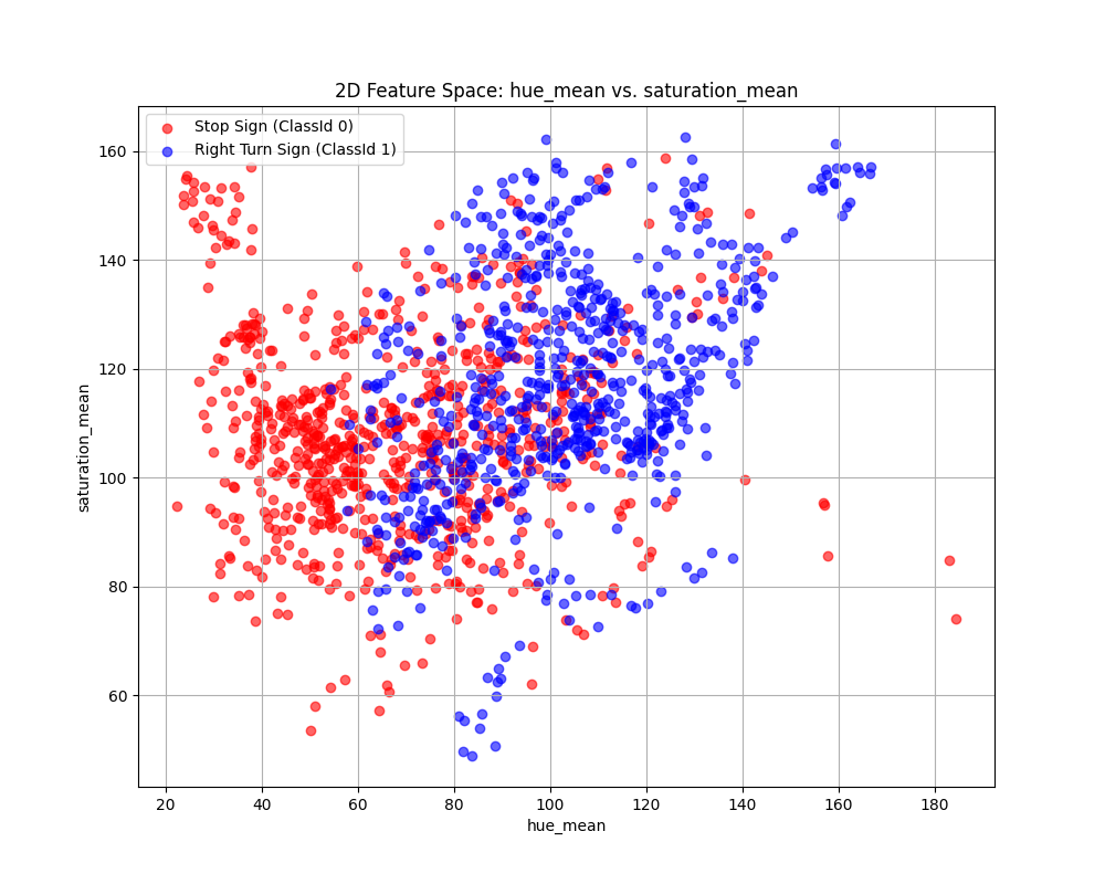
Fig. 12.20 Case_1_KNN_feature_space.png

Case 2 Sample Output

$ python3 tp2_team_3_teamnumber.py Enter the name of the dataset folder: ML_Images Enter the name of the metadata file: img_metadata.csv Enter the name of output csv features file: img_features.csv

Training Metadata DataFrame: Width Height ClassId Path 0 26 29 1 1_00015_00000.png 1 27 30 1 1_00015_00001.png 2 27 30 1 1_00015_00002.png 3 28 31 1 1_00015_00003.png 4 28 30 1 1_00015_00004.png

Features have been extracted and saved to img_features.csv

Feature Dataset Shape: (1469, 10)

Feature Dataset Head: hue_mean hue_std saturation_mean saturation_std ... num_lines has_circle Path ClassId 0 77.5901 74.895838 87.5351 76.634594 ... 0.0 0.0 1_00015_00000.png 1 1 71.8692 73.134396 91.1982 74.631321 ... 0.0 0.0 1_00015_00001.png 1 2 78.3621 73.230186 91.6578 76.665620 ... 0.0 0.0 1_00015_00002.png 1 3 77.3715 71.860282 92.6498 75.498783 ... 0.0 0.0 1_00015_00003.png 1 4 81.7215 70.873320 101.1194 77.180979 ... 0.0 0.0 1_00015_00004.png 1

[5 rows x 10 columns]

Enter the column to use as the x-axis feature: value_mean

Enter the column to use as the y-axis feature: num_lines

Scatter plot saved to KNN_feature_space.png

Fig. 12.21 Case_2_KNN_feature_space.png

Case 3 Sample Output

$ python3 tp2_team_3_teamnumber.py Enter the name of the dataset folder: ML_Images Enter the name of the metadata file: img_metadata.csv Enter the name of output csv features file: img_features.csv

Training Metadata DataFrame: Width Height ClassId Path 0 26 29 1 1_00015_00000.png 1 27 30 1 1_00015_00001.png 2 27 30 1 1_00015_00002.png 3 28 31 1 1_00015_00003.png 4 28 30 1 1_00015_00004.png

Features have been extracted and saved to img_features.csv

Feature Dataset Shape: (1469, 10)

Feature Dataset Head: hue_mean hue_std saturation_mean saturation_std ... num_lines has_circle Path ClassId 0 77.5901 74.895838 87.5351 76.634594 ... 0.0 0.0 1_00015_00000.png 1 1 71.8692 73.134396 91.1982 74.631321 ... 0.0 0.0 1_00015_00001.png 1 2 78.3621 73.230186 91.6578 76.665620 ... 0.0 0.0 1_00015_00002.png 1 3 77.3715 71.860282 92.6498 75.498783 ... 0.0 0.0 1_00015_00003.png 1 4 81.7215 70.873320 101.1194 77.180979 ... 0.0 0.0 1_00015_00004.png 1

[5 rows x 10 columns]

Enter the column to use as the x-axis feature: hue_mean

Enter the column to use as the y-axis feature: hue_std

Scatter plot saved to KNN_feature_space.png

Fig. 12.22 Case_3_KNN_feature_space.png

Table 12.11 Deliverables

Deliverables	Description
tp2_team_3_teamnumber.pdf	Flowchart(s) for this task.
tp2_team_3_teamnumber.py	Your completed Python code.