\[ \begin{align}\begin{aligned}\newcommand\blank{~\underline{\hspace{1.2cm}}~}\\% Bold symbols (vectors) \newcommand\bs[1]{\mathbf{#1}}\\% Differential \newcommand\dd[2][]{\mathrm{d}^{#1}{#2}} % use as \dd, \dd{x}, or \dd[2]{x}\\% Poor man's siunitx \newcommand\unit[1]{\mathrm{#1}} \newcommand\num[1]{#1} \newcommand\qty[2]{#1~\unit{#2}}\\\newcommand\per{/} \newcommand\squared{{}^2} \newcommand\cubed{{}^3} % % Scale \newcommand\milli{\unit{m}} \newcommand\centi{\unit{c}} \newcommand\kilo{\unit{k}} \newcommand\mega{\unit{M}} % % Percent \newcommand\percent{\unit{{\kern-4mu}\%}} % % Angle \newcommand\radian{\unit{rad}} \newcommand\degree{\unit{{\kern-4mu}^\circ}} % % Time \newcommand\second{\unit{s}} \newcommand\s{\second} \newcommand\minute{\unit{min}} \newcommand\hour{\unit{h}} % % Distance \newcommand\meter{\unit{m}} \newcommand\m{\meter} \newcommand\inch{\unit{in}} \newcommand\foot{\unit{ft}} % % Force \newcommand\newton{\unit{N}} \newcommand\kip{\unit{kip}} % kilopound in "freedom" units - edit made by Sri % % Mass \newcommand\gram{\unit{g}} \newcommand\g{\gram} \newcommand\kilogram{\unit{kg}} \newcommand\kg{\kilogram} \newcommand\grain{\unit{grain}} \newcommand\ounce{\unit{oz}} \newcommand\pound{\unit{lbs}} % % Temperature \newcommand\kelvin{\unit{K}} \newcommand\K{\kelvin} \newcommand\celsius{\unit{{\kern-4mu}^\circ C}} \newcommand\C{\celsius} \newcommand\fahrenheit{\unit{{\kern-4mu}^\circ F}} \newcommand\F{\fahrenheit} % % Area \newcommand\sqft{\unit{sq\,\foot}} % square foot % % Volume \newcommand\liter{\unit{L}} \newcommand\gallon{\unit{gal}} % % Frequency \newcommand\hertz{\unit{Hz}} \newcommand\rpm{\unit{rpm}} % % Voltage \newcommand\volt{\unit{V}} \newcommand\V{\volt} \newcommand\millivolt{\milli\volt} \newcommand\mV{\milli\volt} \newcommand\kilovolt{\kilo\volt} \newcommand\kV{\kilo\volt} % % Current \newcommand\ampere{\unit{A}} \newcommand\A{\ampere} \newcommand\milliampereA{\milli\ampere} \newcommand\mA{\milli\ampere} \newcommand\kiloampereA{\kilo\ampere} \newcommand\kA{\kilo\ampere} % % Resistance \newcommand\ohm{\Omega} \newcommand\milliohm{\milli\ohm} \newcommand\kiloohm{\kilo\ohm} % correct SI spelling \newcommand\kilohm{\kilo\ohm} % "American" spelling used in siunitx \newcommand\megaohm{\mega\ohm} % correct SI spelling \newcommand\megohm{\mega\ohm} % "American" spelling used in siunitx % % Capacitance \newcommand\farad{\unit{F}} \newcommand\F{\farad} \newcommand\microfarad{\micro\farad} \newcommand\muF{\micro\farad} % % Inductance \newcommand\henry{\unit{H}} \newcommand\H{\henry} \newcommand\millihenry{\milli\henry} \newcommand\mH{\milli\henry} % % Power \newcommand\watt{\unit{W}} \newcommand\W{\watt} \newcommand\milliwatt{\milli\watt} \newcommand\mW{\milli\watt} \newcommand\kilowatt{\kilo\watt} \newcommand\kW{\kilo\watt} % % Energy \newcommand\joule{\unit{J}} \newcommand\J{\joule} % % Composite units % % Torque \newcommand\ozin{\unit{\ounce}\,\unit{in}} \newcommand\newtonmeter{\unit{\newton\,\meter}} % % Pressure \newcommand\psf{\unit{psf}} % pounds per square foot \newcommand\pcf{\unit{pcf}} % pounds per cubic foot \newcommand\pascal{\unit{Pa}} \newcommand\Pa{\pascal} \newcommand\ksi{\unit{ksi}} % kilopound per square inch \newcommand\bar{\unit{bar}} \end{aligned}\end{align} \]

Apr 28, 2026 | 719 words | 7 min read

5.2.3. Task 3

Learning Objectives

• Reuse kernel-filtering fundamentals from the previous task in a Gaussian-filter setting.

• Construct a normalized Gaussian kernel using a chosen \(\sigma\).

• Apply Gaussian filtering to grayscale images using padding and sliding windows.

• Explain why Gaussian blur is typically preferred over mean blur for this workflow.

Introduction

In the previous task, you implemented the core kernel workflow: create a kernel, pad the image, slide the kernel, and compute weighted sums. In this task, you will keep that same pipeline and replace the mean kernel with a Gaussian kernel.

Why Blur First?

Blurring helps suppress small pixel-level variation (noise-like detail) so larger shapes and boundaries become easier to analyze in later steps.

Why Gaussian Instead of Mean Blur?

The mean filter gives equal weight to all values in the local window. This smooths the image, but can produce blocky behavior and remove too much structure.

A Gaussian filter still smooths the image, but it gives larger weights to values near the center of the kernel and smaller weights to values farther away. You can think of this as a weighted average where nearby pixels influence the result more than distant pixels.

Note

For easier viewing, we recommend using light mode for the following figures.

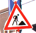
Start from the following small reference image:

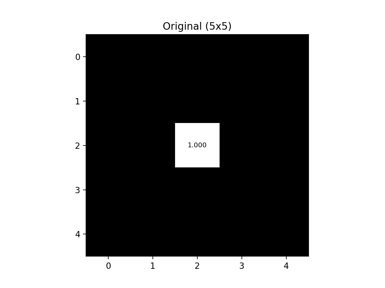
Fig. 5.5 Original Black-White Grid

Mean blur output:

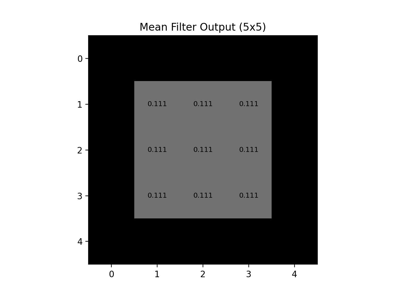
Fig. 5.6 Mean Blur Output

Gaussian blur output:

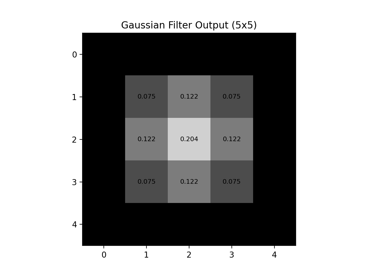
Fig. 5.7 Gaussian Blur Output

Larger comparison:

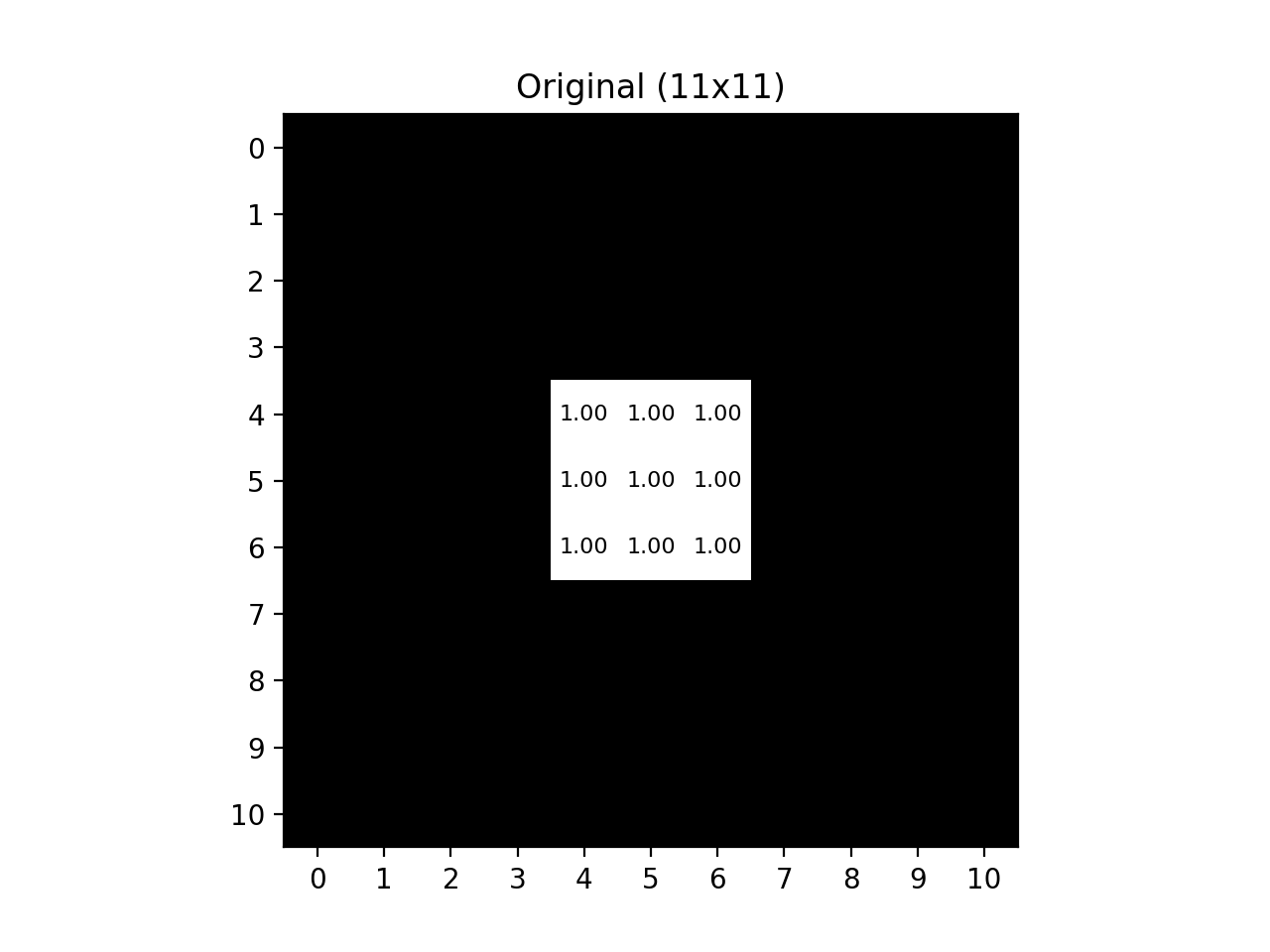
Fig. 5.8 Large Black-White Grid

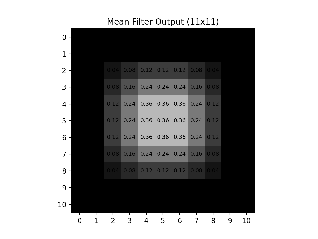
Fig. 5.9 Large Mean Blur Output

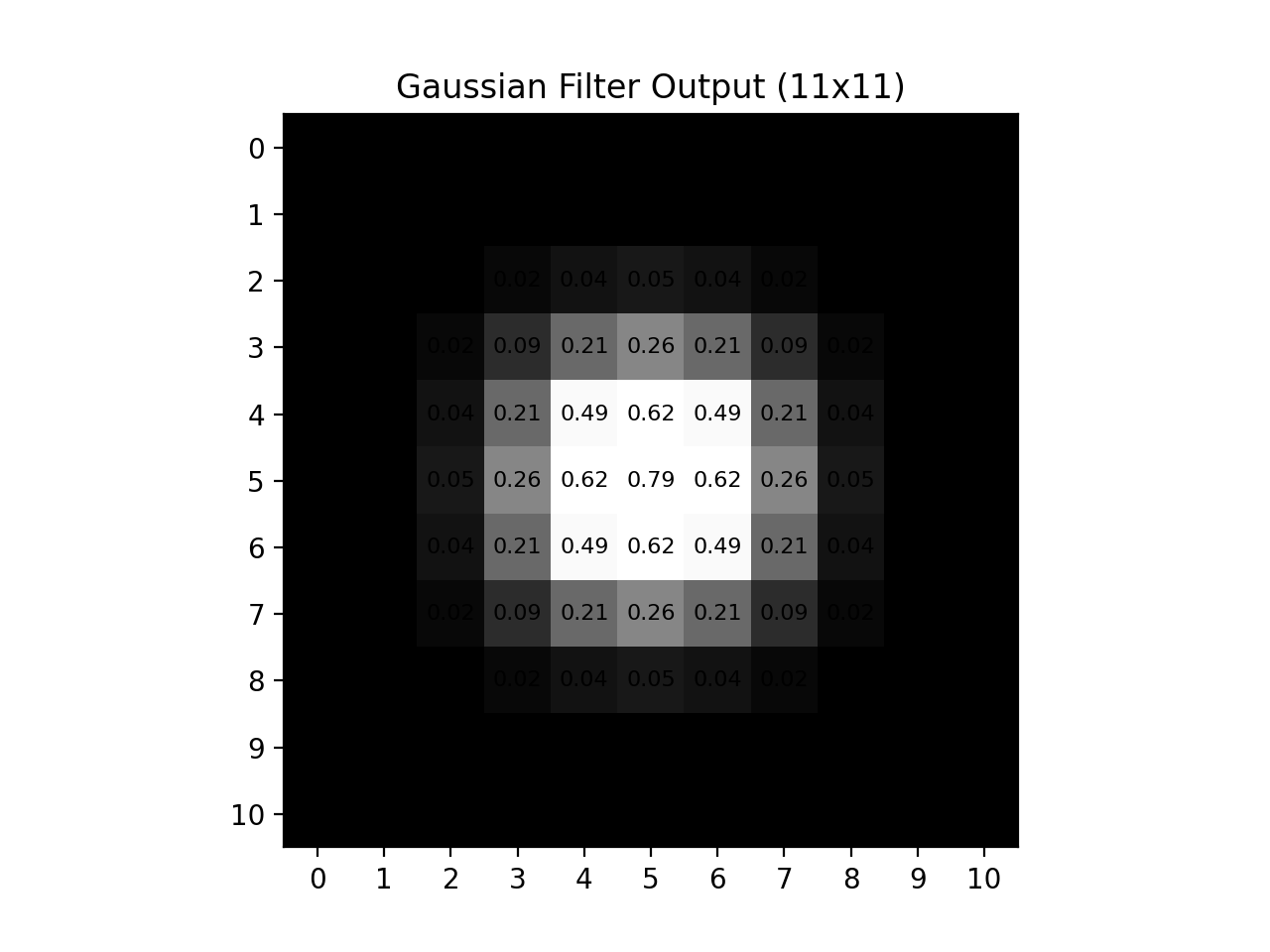
Fig. 5.10 Large Gaussian Blur Output

Both methods blur the original image, so both reduce fine detail. The important difference is how strongly they blur: mean blur is usually more extreme because every pixel in the local window is weighted equally. Gaussian blur is typically less extreme, because center-near pixels get higher weight and farther pixels get lower weight, so more of the original structure is preserved.

Gaussian blur is therefore commonly preferred before feature extraction steps like edge detection, because it smooths noise while preserving larger structures.

Task Instructions

Deliverable Reminder

Create a flowchart of your algorithm and save it as tp1_team_3_teamnumber.pdf. Start your program from a copy of the ENGR133_Python_Template.py template and name it tp1_team_3_teamnumber.py.

You will write two functions, one to build a Gaussian kernel and one to apply it, then use them to blur a user-selected grayscale image. Before you begin, create a folder named ref_images in the same directory as your program and download the reference images listed in Table 5.8 into it.

Table 5.8 Reference Image Download

Reference Image	Download Link
Color Reference A	ref_col_a.png
Color Reference B	ref_col_b.png

Create Gaussian Kernel Function

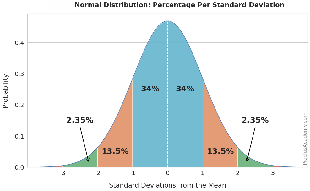
Fig. 5.11 Normal Curve

Create a function named create_gaussian_kernel that takes one parameter, \(\sigma\), and returns a normalized 2D Gaussian kernel as a NumPy array.

Use the 2D Gaussian formula:

(5.8)\[G(x, y) = \frac{1}{2\pi\sigma^2}\cdot e^{-\frac{x^2 + y^2}{2\sigma^2}}\]

Where:

• \(x\) and \(y\) are relative offsets from the kernel center.

• \(\sigma\) controls spread:

  • smaller \(\sigma\) gives a tighter blur

  • larger \(\sigma\) gives a wider blur

Determine kernel size with:

(5.9)\[\text{kernel_size} = 2\times\lceil 3\sigma \rceil + 1\]

This keeps the kernel odd-sized and includes values out to about \(\pm 3\sigma\) from the center.

Requirements:

• \(\sigma\) is a positive float.

• The kernel must be square and odd-sized.

• Normalize the kernel so the sum of all elements is \(1.0\).

• Return a 2D NumPy array of floats.

Note

For this assignment, use \(\sigma = 1\) in main.

Gaussian Filter Function

Create a function named gaussian_filter that takes two parameters, image and \(\sigma\), and returns the Gaussian-blurred image.

Requirements:

• image is a 2D grayscale NumPy array.

• Build the kernel by calling create_gaussian_kernel(sigma).

• Zero-pad the image based on kernel size.

• Slide the kernel across the image with stride \(1\).

• At each output location, compute the weighted sum of the local window.

• Return a NumPy array with the same shape as the input image.

To determine padding width:

(5.10)\[\text{pad_size} = \frac{\text{kernel_size} - 1}{2}\]

Note

Do not modify the original image in place. Write filtered results into a separate output array.

Main Function

Note

You will need the load_img and rgb_to_grayscale functions developed in Section 15.2.2. Copy them into your program.

In your main function, you will need to do the following:

1. Ask the user for an image filename (for example, ref_col_a.png).

2. Load the image from the ref_images folder using load_img.

3. Convert the image to grayscale using rgb_to_grayscale.

4. Apply gaussian_filter with \(\sigma = 1\).

5. Display and save the blurred image.

Sample Output

Test cases for Gaussian kernel creation and filtering workflow. Use the values in Table 5.9 below to test your program.

Table 5.9 Test Cases

Case	image_path
1	ref_col_a.png
2	ref_col_b.png

Ensure your program’s output matches the provided samples exactly. This includes all characters, white space, and punctuation. In the samples, user input is highlighted like this for clarity, but your program should not highlight user input in this way.

Case 1 Sample Output

$ python3 tp1_team_3_teamnumber.py Enter the path to the image file: ref_col_a.png

Fig. 5.12 Case_1_ref_col_a_smooth.png

Case 2 Sample Output

$ python3 tp1_team_3_teamnumber.py Enter the path to the image file: ref_col_b.png

Fig. 5.13 Case_2_ref_col_b_smooth.png

Table 5.10 Deliverables

Deliverables	Description
tp1_team_3_teamnumber.pdf	Flowchart(s) for this task.
tp1_team_3_teamnumber.py	Your completed Python code.