\[ \begin{align}\begin{aligned}\newcommand\blank{~\underline{\hspace{1.2cm}}~}\\% Bold symbols (vectors) \newcommand\bs[1]{\mathbf{#1}}\\% Differential \newcommand\dd[2][]{\mathrm{d}^{#1}{#2}} % use as \dd, \dd{x}, or \dd[2]{x}\\% Poor man's siunitx \newcommand\unit[1]{\mathrm{#1}} \newcommand\num[1]{#1} \newcommand\qty[2]{#1~\unit{#2}}\\\newcommand\per{/} \newcommand\squared{{}^2} \newcommand\cubed{{}^3} % % Scale \newcommand\milli{\unit{m}} \newcommand\centi{\unit{c}} \newcommand\kilo{\unit{k}} \newcommand\mega{\unit{M}} % % Percent \newcommand\percent{\unit{{\kern-4mu}\%}} % % Angle \newcommand\radian{\unit{rad}} \newcommand\degree{\unit{{\kern-4mu}^\circ}} % % Time \newcommand\second{\unit{s}} \newcommand\s{\second} \newcommand\minute{\unit{min}} \newcommand\hour{\unit{h}} % % Distance \newcommand\meter{\unit{m}} \newcommand\m{\meter} \newcommand\inch{\unit{in}} \newcommand\foot{\unit{ft}} % % Force \newcommand\newton{\unit{N}} \newcommand\kip{\unit{kip}} % kilopound in "freedom" units - edit made by Sri % % Mass \newcommand\gram{\unit{g}} \newcommand\g{\gram} \newcommand\kilogram{\unit{kg}} \newcommand\kg{\kilogram} \newcommand\grain{\unit{grain}} \newcommand\ounce{\unit{oz}} \newcommand\pound{\unit{lbs}} % % Temperature \newcommand\kelvin{\unit{K}} \newcommand\K{\kelvin} \newcommand\celsius{\unit{{\kern-4mu}^\circ C}} \newcommand\C{\celsius} \newcommand\fahrenheit{\unit{{\kern-4mu}^\circ F}} \newcommand\F{\fahrenheit} % % Area \newcommand\sqft{\unit{sq\,\foot}} % square foot % % Volume \newcommand\liter{\unit{L}} \newcommand\gallon{\unit{gal}} % % Frequency \newcommand\hertz{\unit{Hz}} \newcommand\rpm{\unit{rpm}} % % Voltage \newcommand\volt{\unit{V}} \newcommand\V{\volt} \newcommand\millivolt{\milli\volt} \newcommand\mV{\milli\volt} \newcommand\kilovolt{\kilo\volt} \newcommand\kV{\kilo\volt} % % Current \newcommand\ampere{\unit{A}} \newcommand\A{\ampere} \newcommand\milliampereA{\milli\ampere} \newcommand\mA{\milli\ampere} \newcommand\kiloampereA{\kilo\ampere} \newcommand\kA{\kilo\ampere} % % Resistance \newcommand\ohm{\Omega} \newcommand\milliohm{\milli\ohm} \newcommand\kiloohm{\kilo\ohm} % correct SI spelling \newcommand\kilohm{\kilo\ohm} % "American" spelling used in siunitx \newcommand\megaohm{\mega\ohm} % correct SI spelling \newcommand\megohm{\mega\ohm} % "American" spelling used in siunitx % % Capacitance \newcommand\farad{\unit{F}} \newcommand\F{\farad} \newcommand\microfarad{\micro\farad} \newcommand\muF{\micro\farad} % % Inductance \newcommand\henry{\unit{H}} \newcommand\H{\henry} \newcommand\millihenry{\milli\henry} \newcommand\mH{\milli\henry} % % Power \newcommand\watt{\unit{W}} \newcommand\W{\watt} \newcommand\milliwatt{\milli\watt} \newcommand\mW{\milli\watt} \newcommand\kilowatt{\kilo\watt} \newcommand\kW{\kilo\watt} % % Energy \newcommand\joule{\unit{J}} \newcommand\J{\joule} % % Composite units % % Torque \newcommand\ozin{\unit{\ounce}\,\unit{in}} \newcommand\newtonmeter{\unit{\newton\,\meter}} % % Pressure \newcommand\psf{\unit{psf}} % pounds per square foot \newcommand\pcf{\unit{pcf}} % pounds per cubic foot \newcommand\pascal{\unit{Pa}} \newcommand\Pa{\pascal} \newcommand\ksi{\unit{ksi}} % kilopound per square inch \newcommand\bar{\unit{bar}} \end{aligned}\end{align} \]

Apr 28, 2026 | 751 words | 8 min read

6.2.3. Task 3

Learning Objectives

• Use pandas to work with tabular CSV data

• Use the pandas library to read data, apply functions, and build a scaled final feature dataset

• Visualize the relationship between features using a scatter plot, with points colored by class label

• Understand the purpose of feature scaling and how to apply it to a dataset

Introduction

In this task, you will use the features extracted in the previous task. Your script will read the CSV features file, apply feature scaling, and plot the relationship between features.

This task will require you to use the pandas library, which is a powerful tool for data manipulation and analysis in Python. If you are unfamiliar with pandas, refer to the materials provided in Section 6.1.1.

Feature scaling standardizes each numeric feature by subtracting its mean and dividing by its standard deviation. You may notice that scatter plots of scaled features look similar to those of the original features, but the axes will differ: the scaled axes will be centered at 0 with a standard deviation of 1, while the original axes may span a wider range. Feature scaling does not change the relationship between features; it only changes their scale. Ensuring all features are on a similar scale can help certain machine learning algorithms perform better.

Task Instructions

Deliverable Reminder

Create a flowchart of your algorithm and save it as tp2_team_3_teamnumber.pdf. Include all flowcharts in your final report.

Feature Scaling Function

Create a function named scale_features:

Arguments:

• A pandas DataFrame

• A list of feature column names (as strings) to be scaled

Returns:

• None (the function modifies the DataFrame in place)

For each column in the list of feature column names, calculate the mean and standard deviation of that column. Then, scale the value in every row of that column using the formula:

(6.4)\[x_{scaled} = \frac{x - \mu}{\sigma}\]

Where:

• \(x\) is the original feature value

• \(\mu\) is the mean of the entire feature column

• \(\sigma\) is the standard deviation of the entire feature column

Your function should NOT return anything. Instead, it should modify the input DataFrame in place. After calling the function, the original DataFrame will have its specified feature columns scaled without creating a new DataFrame object, thus saving memory.

Main Function

1. The main function should first collect the following inputs from the user:

   • the path to the image features CSV file (the output from Task 2)

   • whether to apply feature scaling (yes/no)

2. The function should load the features CSV file into a pandas DataFrame using pd.read_csv().

3. If the user chose to apply feature scaling, call the scale_features function on the DataFrame with the appropriate feature column names.

   • You can hardcode the list of feature column names in your code since you know which features you extracted in Task 2.

   • If the user chose not to apply feature scaling, simply proceed with the original DataFrame without modification.

   • Add print statements to indicate whether feature scaling is being applied or not, and to confirm when the scaling process is complete.

4. Display the size and head of the dataset to show the result with or without scaling.

5. Prompt the user for two or three feature names which will be used for plotting. See the sample output below for an example of how to do this.

   • If no z-axis feature is provided, only plot the two features in a 2D scatter plot.

   • If a z-axis feature is provided, create a 3D scatter plot. See the docs for matplotlib to learn how to create 3D scatter plots.

6. Create the feature scatter plot. Separate the dataset into two groups based on the ClassId column. Then call plt.scatter once for each group, using the c parameter to assign explicit string colors: c='red' for deer warning signs (ClassId 0) and c='blue' for left turn ahead signs (ClassId 1). Set alpha=0.6 to make the points semi-transparent. Assign a descriptive label to each call so that a legend can be generated with plt.legend(). Label the axes appropriately.

Hint

You may need to use matplotlib.use('TkAgg') at the beginning of your script to ensure that the plots display correctly on all platforms.

7. Save the scatter plot image to "KNN_feature_space.png" using plt.savefig. Print a message confirming the filename where the plot was saved.

Save your program as tp2_team_3_teamnumber.py.

Sample Output

Use the values in Table 6.9 below to test your program.

Table 6.9 Test Cases

Case	features_csv_path	apply_scaling	xfeature	yfeature	zfeature
1	img_features.csv	No	hue_mean	saturation_mean
2	img_features.csv	No	hue_mean	saturation_mean	value_mean
3	img_features.csv	Yes	hue_mean	saturation_mean	value_mean
4	img_features.csv	No	hue_mean	has_triangle	has_circle
5	img_features.csv	Yes	hue_mean	has_triangle	has_circle
6	img_features.csv	No	hue_std	number_lines
7	img_features.csv	Yes	hue_std	number_lines

Ensure your program’s output matches the provided samples exactly. This includes all characters, white space, and punctuation. In the samples, user input is highlighted like this for clarity, but your program should not highlight user input in this way.

Case 1 Sample Output

$ python3 tp2_team_3_teamnumber.py Enter the name of CSV image features file: img_features.csv Do you want to apply feature scaling? (yes/no): No Proceeding without feature scaling.

Feature Dataset Shape: (1080, 11)

Feature Dataset Head: hue_mean hue_std saturation_mean saturation_std value_mean value_std number_lines has_circle has_triangle Path ClassId 0 153.2073 61.059767 91.9556 40.786746 17.8427 19.008287 2.0 0.0 0.0 0001.png 0 1 81.7387 87.964121 151.8222 55.362343 126.3639 91.494998 49.0 1.0 0.0 0002.png 1 2 153.4376 57.676740 95.8184 38.068961 21.2990 22.463993 1.0 0.0 0.0 0003.png 0 3 82.5612 83.471986 147.9150 63.461210 127.8036 90.167103 42.0 1.0 0.0 0004.png 1 4 154.4448 57.903069 95.9104 40.238663 24.2915 24.985162 1.0 0.0 0.0 0005.png 0

Enter the column to use as the x-axis feature: hue_mean

Enter the column to use as the y-axis feature: saturation_mean

Enter the column to use as the z-axis feature (or press Enter to skip):

Scatter plot saved to KNN_feature_space.png

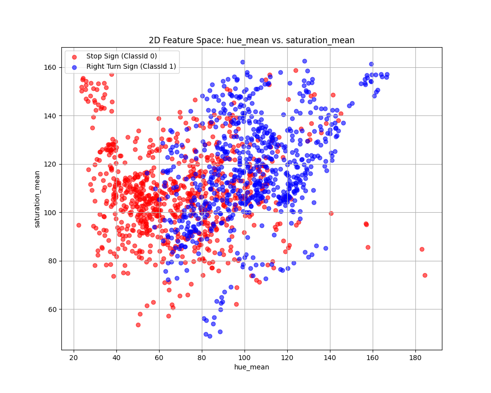
Fig. 6.11 Case_1_KNN_feature_space.png

Case 2 Sample Output

$ python3 tp2_team_3_teamnumber.py Enter the name of CSV image features file: img_features.csv Do you want to apply feature scaling? (yes/no): No Proceeding without feature scaling.

Feature Dataset Shape: (1080, 11)

Feature Dataset Head: hue_mean hue_std saturation_mean saturation_std value_mean value_std number_lines has_circle has_triangle Path ClassId 0 153.2073 61.059767 91.9556 40.786746 17.8427 19.008287 2.0 0.0 0.0 0001.png 0 1 81.7387 87.964121 151.8222 55.362343 126.3639 91.494998 49.0 1.0 0.0 0002.png 1 2 153.4376 57.676740 95.8184 38.068961 21.2990 22.463993 1.0 0.0 0.0 0003.png 0 3 82.5612 83.471986 147.9150 63.461210 127.8036 90.167103 42.0 1.0 0.0 0004.png 1 4 154.4448 57.903069 95.9104 40.238663 24.2915 24.985162 1.0 0.0 0.0 0005.png 0

Enter the column to use as the x-axis feature: hue_mean

Enter the column to use as the y-axis feature: saturation_mean

Enter the column to use as the z-axis feature (or press Enter to skip): value_mean

Scatter plot saved to KNN_feature_space.png

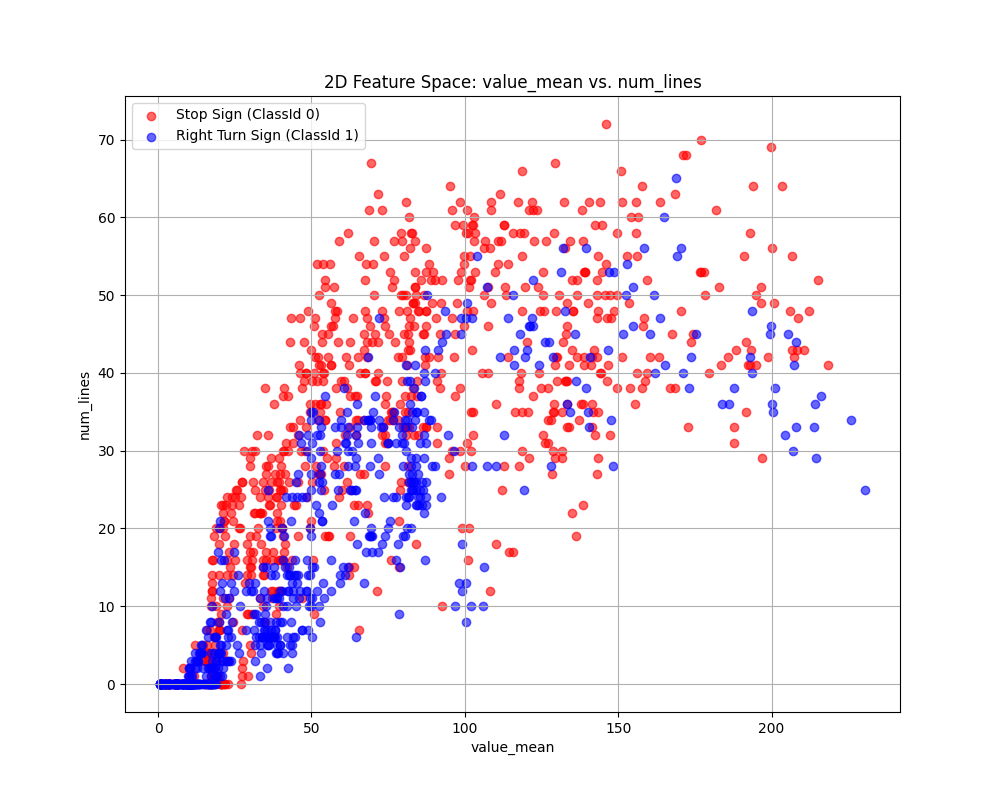
Fig. 6.12 Case_2_KNN_feature_space.png

Case 3 Sample Output

$ python3 tp2_team_3_teamnumber.py Enter the name of CSV image features file: img_features.csv Do you want to apply feature scaling? (yes/no): Yes Applying feature scaling to the dataset... Feature scaling applied successfully.

Feature Dataset Shape: (1080, 11)

Feature Dataset Head: hue_mean hue_std saturation_mean saturation_std value_mean value_std number_lines has_circle has_triangle Path ClassId 0 1.354593 -0.188960 -0.428141 -1.575216 -0.757578 -0.714781 -0.875255 -0.766610 -0.36651 0001.png 0 1 -0.356171 1.150234 1.199187 -0.755132 0.887890 1.359262 1.891979 1.303237 -0.36651 0002.png 1 2 1.360106 -0.357353 -0.323140 -1.728130 -0.705171 -0.615903 -0.934132 -0.766610 -0.36651 0003.png 0 3 -0.336483 0.926633 1.092979 -0.299456 0.909719 1.321268 1.479838 1.303237 -0.36651 0004.png 1 4 1.384215 -0.346088 -0.320639 -1.606054 -0.659797 -0.543766 -0.934132 -0.766610 -0.36651 0005.png 0

Enter the column to use as the x-axis feature: hue_mean

Enter the column to use as the y-axis feature: saturation_mean

Enter the column to use as the z-axis feature (or press Enter to skip): value_mean

Scatter plot saved to KNN_feature_space.png

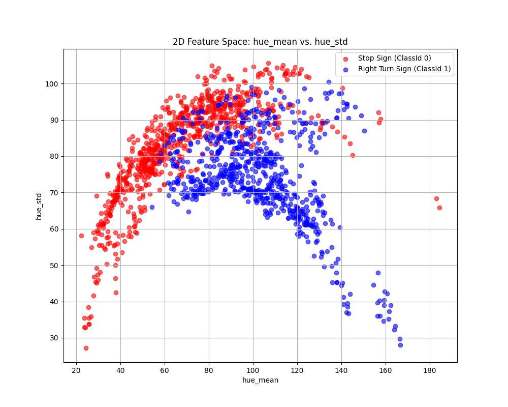
Fig. 6.13 Case_3_KNN_feature_space.png

Case 4 Sample Output

$ python3 tp2_team_3_teamnumber.py Enter the name of CSV image features file: img_features.csv Do you want to apply feature scaling? (yes/no): No Proceeding without feature scaling.

Feature Dataset Shape: (1080, 11)

Feature Dataset Head: hue_mean hue_std saturation_mean saturation_std value_mean value_std number_lines has_circle has_triangle Path ClassId 0 153.2073 61.059767 91.9556 40.786746 17.8427 19.008287 2.0 0.0 0.0 0001.png 0 1 81.7387 87.964121 151.8222 55.362343 126.3639 91.494998 49.0 1.0 0.0 0002.png 1 2 153.4376 57.676740 95.8184 38.068961 21.2990 22.463993 1.0 0.0 0.0 0003.png 0 3 82.5612 83.471986 147.9150 63.461210 127.8036 90.167103 42.0 1.0 0.0 0004.png 1 4 154.4448 57.903069 95.9104 40.238663 24.2915 24.985162 1.0 0.0 0.0 0005.png 0

Enter the column to use as the x-axis feature: hue_mean

Enter the column to use as the y-axis feature: has_triangle

Enter the column to use as the z-axis feature (or press Enter to skip): has_circle

Scatter plot saved to KNN_feature_space.png

Fig. 6.14 Case_4_KNN_feature_space.png

Case 5 Sample Output

$ python3 tp2_team_3_teamnumber.py Enter the name of CSV image features file: img_features.csv Do you want to apply feature scaling? (yes/no): Yes Applying feature scaling to the dataset... Feature scaling applied successfully.

Feature Dataset Shape: (1080, 11)

Feature Dataset Head: hue_mean hue_std saturation_mean saturation_std value_mean value_std number_lines has_circle has_triangle Path ClassId 0 1.354593 -0.188960 -0.428141 -1.575216 -0.757578 -0.714781 -0.875255 -0.766610 -0.36651 0001.png 0 1 -0.356171 1.150234 1.199187 -0.755132 0.887890 1.359262 1.891979 1.303237 -0.36651 0002.png 1 2 1.360106 -0.357353 -0.323140 -1.728130 -0.705171 -0.615903 -0.934132 -0.766610 -0.36651 0003.png 0 3 -0.336483 0.926633 1.092979 -0.299456 0.909719 1.321268 1.479838 1.303237 -0.36651 0004.png 1 4 1.384215 -0.346088 -0.320639 -1.606054 -0.659797 -0.543766 -0.934132 -0.766610 -0.36651 0005.png 0

Enter the column to use as the x-axis feature: hue_mean

Enter the column to use as the y-axis feature: has_triangle

Enter the column to use as the z-axis feature (or press Enter to skip): has_circle

Scatter plot saved to KNN_feature_space.png

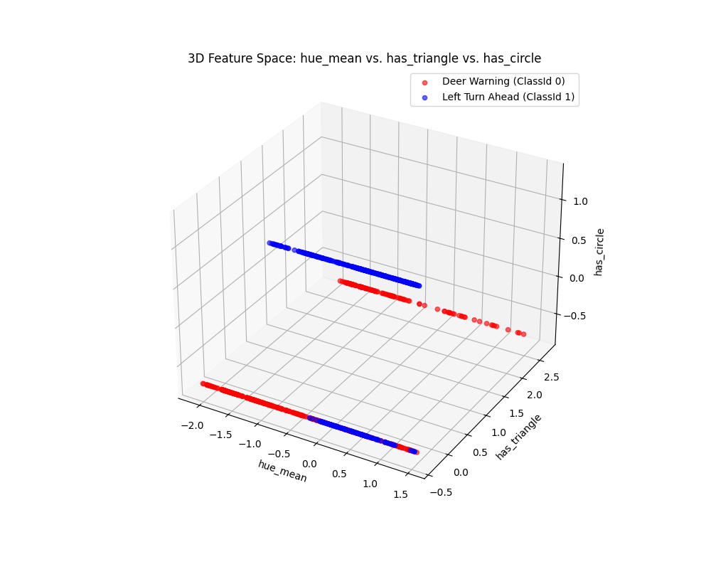
Fig. 6.15 Case_5_KNN_feature_space.png

Case 6 Sample Output

$ python3 tp2_team_3_teamnumber.py Enter the name of CSV image features file: img_features.csv Do you want to apply feature scaling? (yes/no): No Proceeding without feature scaling.

Feature Dataset Shape: (1080, 11)

Feature Dataset Head: hue_mean hue_std saturation_mean saturation_std value_mean value_std number_lines has_circle has_triangle Path ClassId 0 153.2073 61.059767 91.9556 40.786746 17.8427 19.008287 2.0 0.0 0.0 0001.png 0 1 81.7387 87.964121 151.8222 55.362343 126.3639 91.494998 49.0 1.0 0.0 0002.png 1 2 153.4376 57.676740 95.8184 38.068961 21.2990 22.463993 1.0 0.0 0.0 0003.png 0 3 82.5612 83.471986 147.9150 63.461210 127.8036 90.167103 42.0 1.0 0.0 0004.png 1 4 154.4448 57.903069 95.9104 40.238663 24.2915 24.985162 1.0 0.0 0.0 0005.png 0

Enter the column to use as the x-axis feature: hue_std

Enter the column to use as the y-axis feature: number_lines

Enter the column to use as the z-axis feature (or press Enter to skip):

Scatter plot saved to KNN_feature_space.png

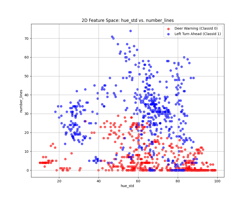
Fig. 6.16 Case_6_KNN_feature_space.png

Case 7 Sample Output

$ python3 tp2_team_3_teamnumber.py Enter the name of CSV image features file: img_features.csv Do you want to apply feature scaling? (yes/no): Yes Applying feature scaling to the dataset... Feature scaling applied successfully.

Feature Dataset Shape: (1080, 11)

Feature Dataset Head: hue_mean hue_std saturation_mean saturation_std value_mean value_std number_lines has_circle has_triangle Path ClassId 0 1.354593 -0.188960 -0.428141 -1.575216 -0.757578 -0.714781 -0.875255 -0.766610 -0.36651 0001.png 0 1 -0.356171 1.150234 1.199187 -0.755132 0.887890 1.359262 1.891979 1.303237 -0.36651 0002.png 1 2 1.360106 -0.357353 -0.323140 -1.728130 -0.705171 -0.615903 -0.934132 -0.766610 -0.36651 0003.png 0 3 -0.336483 0.926633 1.092979 -0.299456 0.909719 1.321268 1.479838 1.303237 -0.36651 0004.png 1 4 1.384215 -0.346088 -0.320639 -1.606054 -0.659797 -0.543766 -0.934132 -0.766610 -0.36651 0005.png 0

Enter the column to use as the x-axis feature: hue_std

Enter the column to use as the y-axis feature: number_lines

Enter the column to use as the z-axis feature (or press Enter to skip):

Scatter plot saved to KNN_feature_space.png

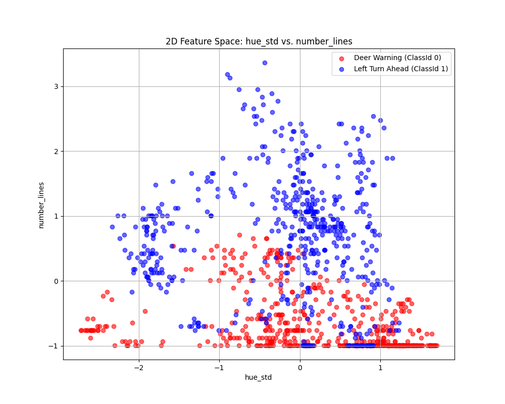
Fig. 6.17 Case_7_KNN_feature_space.png

Table 6.10 Deliverables

Deliverables	Description
tp2_team_3_teamnumber.pdf	Flowchart(s) for this task.
tp2_team_3_teamnumber.py	Your completed Python code.