\[ \begin{align}\begin{aligned}\newcommand\blank{~\underline{\hspace{1.2cm}}~}\\% Bold symbols (vectors) \newcommand\bs[1]{\mathbf{#1}}\\% Differential \newcommand\dd[2][]{\mathrm{d}^{#1}{#2}} % use as \dd, \dd{x}, or \dd[2]{x}\\% Poor man's siunitx \newcommand\unit[1]{\mathrm{#1}} \newcommand\num[1]{#1} \newcommand\qty[2]{#1~\unit{#2}}\\\newcommand\per{/} \newcommand\squared{{}^2} \newcommand\cubed{{}^3} % % Scale \newcommand\milli{\unit{m}} \newcommand\centi{\unit{c}} \newcommand\kilo{\unit{k}} \newcommand\mega{\unit{M}} % % Percent \newcommand\percent{\unit{{\kern-4mu}\%}} % % Angle \newcommand\radian{\unit{rad}} \newcommand\degree{\unit{{\kern-4mu}^\circ}} % % Time \newcommand\second{\unit{s}} \newcommand\s{\second} \newcommand\minute{\unit{min}} \newcommand\hour{\unit{h}} % % Distance \newcommand\meter{\unit{m}} \newcommand\m{\meter} \newcommand\inch{\unit{in}} \newcommand\foot{\unit{ft}} % % Force \newcommand\newton{\unit{N}} \newcommand\kip{\unit{kip}} % kilopound in "freedom" units - edit made by Sri % % Mass \newcommand\gram{\unit{g}} \newcommand\g{\gram} \newcommand\kilogram{\unit{kg}} \newcommand\kg{\kilogram} \newcommand\grain{\unit{grain}} \newcommand\ounce{\unit{oz}} \newcommand\pound{\unit{lbs}} % % Temperature \newcommand\kelvin{\unit{K}} \newcommand\K{\kelvin} \newcommand\celsius{\unit{{\kern-4mu}^\circ C}} \newcommand\C{\celsius} \newcommand\fahrenheit{\unit{{\kern-4mu}^\circ F}} \newcommand\F{\fahrenheit} % % Area \newcommand\sqft{\unit{sq\,\foot}} % square foot % % Volume \newcommand\liter{\unit{L}} \newcommand\gallon{\unit{gal}} % % Frequency \newcommand\hertz{\unit{Hz}} \newcommand\rpm{\unit{rpm}} % % Voltage \newcommand\volt{\unit{V}} \newcommand\V{\volt} \newcommand\millivolt{\milli\volt} \newcommand\mV{\milli\volt} \newcommand\kilovolt{\kilo\volt} \newcommand\kV{\kilo\volt} % % Current \newcommand\ampere{\unit{A}} \newcommand\A{\ampere} \newcommand\milliampereA{\milli\ampere} \newcommand\mA{\milli\ampere} \newcommand\kiloampereA{\kilo\ampere} \newcommand\kA{\kilo\ampere} % % Resistance \newcommand\ohm{\Omega} \newcommand\milliohm{\milli\ohm} \newcommand\kiloohm{\kilo\ohm} % correct SI spelling \newcommand\kilohm{\kilo\ohm} % "American" spelling used in siunitx \newcommand\megaohm{\mega\ohm} % correct SI spelling \newcommand\megohm{\mega\ohm} % "American" spelling used in siunitx % % Capacitance \newcommand\farad{\unit{F}} \newcommand\F{\farad} \newcommand\microfarad{\micro\farad} \newcommand\muF{\micro\farad} % % Inductance \newcommand\henry{\unit{H}} \newcommand\H{\henry} \newcommand\millihenry{\milli\henry} \newcommand\mH{\milli\henry} % % Power \newcommand\watt{\unit{W}} \newcommand\W{\watt} \newcommand\milliwatt{\milli\watt} \newcommand\mW{\milli\watt} \newcommand\kilowatt{\kilo\watt} \newcommand\kW{\kilo\watt} % % Energy \newcommand\joule{\unit{J}} \newcommand\J{\joule} % % Composite units % % Torque \newcommand\ozin{\unit{\ounce}\,\unit{in}} \newcommand\newtonmeter{\unit{\newton\,\meter}} % % Pressure \newcommand\psf{\unit{psf}} % pounds per square foot \newcommand\pcf{\unit{pcf}} % pounds per cubic foot \newcommand\pascal{\unit{Pa}} \newcommand\Pa{\pascal} \newcommand\ksi{\unit{ksi}} % kilopound per square inch \newcommand\bar{\unit{bar}} \end{aligned}\end{align} \]

Apr 28, 2026 | 1029 words | 10 min read

15.3.2. Task 2

Learning Objectives

• Use Python file I/O and modern libraries to load and handle image data.

• Develop an understanding of Python libraries for image processing.

• Apply mathematical methods to image data to perform image-based operations.

• Navigate and manipulate image data programmatically by iterating over pixels, regions, or image arrays.

Introduction

Object and feature detection are core problems in computer vision (CV) and are used in many real-world applications. For example, self-driving cars rely on detecting traffic signs to understand their surroundings, improve cruise control, and plan safe routes. In materials engineering, computer vision techniques are used to identify features such as phases and grain boundaries in metal alloys to better understand their performance. Feature detection is also important in medical imaging, such as Magnetic Resonance Imaging (MRI), where it can help identify details that are difficult for the human eye to see. In recent years, advances in neural networks have greatly improved the speed and accuracy of object detection, in some cases outperforming humans on tasks like recognizing handwritten numbers.

Template matching is a widely used computer vision method for object detection. It works by searching an image for regions that closely match a predefined template, and its simplicity makes it one of the most accessible techniques to understand and implement.

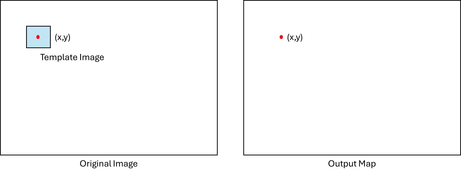
Fig. 15.17 Illustration of template matching

During the matching process, your code will slide the template across the source image one pixel at a time. At each position, it will calculate a numerical score that shows how closely the template matches that part of the image. These scores are combined to create an output map, which can then be used to determine the most likely location of the object. For this task, you will apply template matching to locate Waldo, the famously hidden character, within several busy, visually complex scenes.

Task Instructions

Design a program that loads in a scene image and template image, converts them to grayscale, and then uses the SSD method (described below) to find the location of the template image within the scene image. The program should then display the original scene image with a red rectangle around the location of the template image, and print the x and y coordinates of the template image within the scene image.

The program should be modular, with separate functions for loading images, converting to grayscale, calculating the SSD output map, and drawing the rectangle on the original image. These functions are described in detail below. The main function should orchestrate these steps by collecting user input, calling each function in sequence, and printing the final output to the user.

Develop a flowchart of your design and save it as py5_ind_2_username.pdf. Then start writing your program from a copy of the ENGR133_Python_Template.py Python template. Name this program py5_ind_2_username.py.

Note

For this assignment, please revisit Section 15.1.1 and read the documentation thoroughly. You will need to use the PIL, numpy, and matplotlib.pyplot libraries to load images, manipulate image arrays, and display images, respectively.

Table 15.14 Scene and Template Images

Scene Number	Scene Image	Template Image
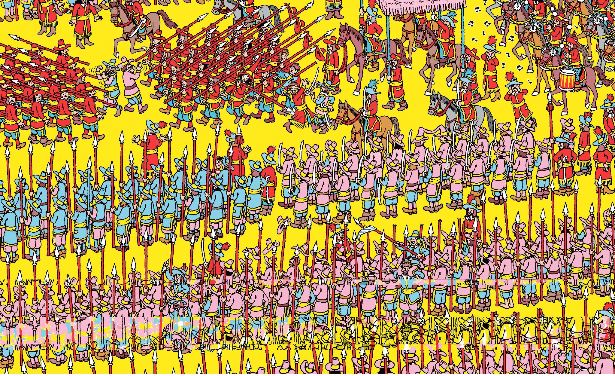
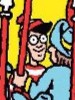
Scene 1	scene_1.jpg	template_1.jpg
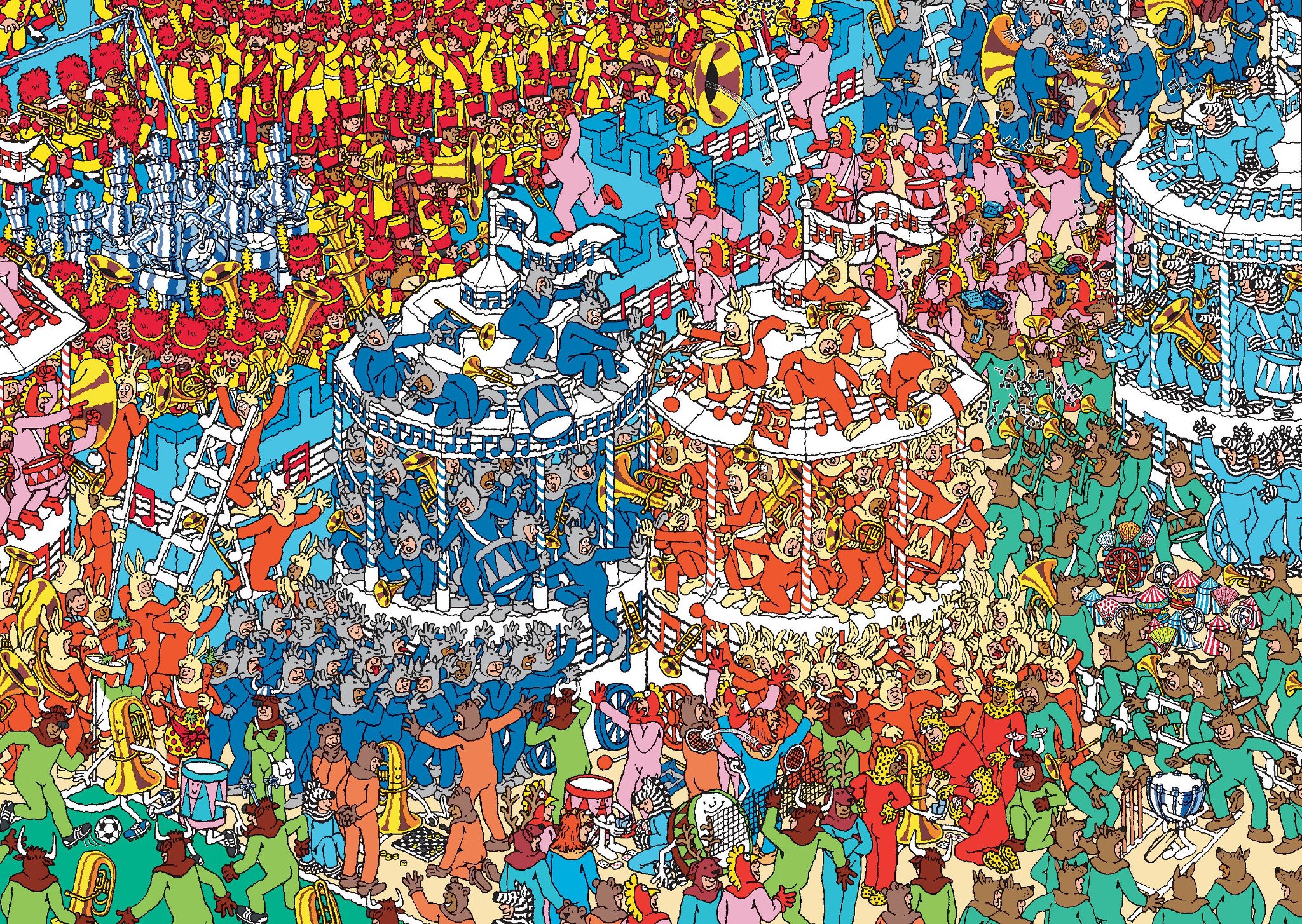
Scene 2	scene_2.jpg	template_2.jpg
Scene 3	scene_3.jpg	template_3.jpg

Step 1: Load images using load_img and rgb_to_grayscale functions

Create a function to load the image of Waldo (template image) and the scene image (source image). Use PIL.Image.open to load each image and convert it to a NumPy array. See the official docs for usage details. Prepare the image for analysis by removing additional channels, normalizing the pixel values, and linearizing the pixels in the image. Use the function load_img created in Team Task 2.

Convert the image to grayscale using the function rgb_to_grayscale created in Team Task 2.

Step 2: SSD Function

Next, we are going to create a function that uses the Sum of Squared Differences (SSD) method to determine the location of the template image within the scene image. Call this function ssd, which takes the grayscale scene image as the first input and the grayscale template image as the second input, and returns a single array, an output map of R values.

The \(R\) value represents the similarity between the template and the scene image at each location – a smaller value indicates a closer match. The equation is:

(15.9)\[R(i,j) = \sum_{k=0}^{w-1}{(\sum_{l=0}^{h-1}(I(i+k, j+l) - T(k, l))^2)}\]

Where

• \(I\) is a matrix representing the scene image;

• \(T\) is a matrix representing the template image;

• \(i,j\) are the indexing of the output map;

• \(k,l\) are the indexing of the template;

• \(w,h\) are the width and height of the template image, in pixels.

The output \(R\) is a matrix of these scores across the scene image. At each position \((i,j)\), the region of \(I\) compared against the template is the same size as the template.

Begin by initializing a blank output map to store the \(R\) values.

Note

This task does not require edge case handling; do not process positions where the template would extend beyond the boundary of the scene image.

Step 3: Draw Rectangle Function

Finally, create a function that displays the original scene image with a rectangle around the best-matching template location. Name this function draw_rectangle, taking the original scene image (NumPy array), the original template image (NumPy array), and the \(R\) output map from ssd as its three inputs. The function returns the x and y location of the template within the scene image.

To do this, get the width and height of the template, and then find the x and y location of the minimum \(R\) value in the output map.

Use matplotlib.pyplot to display the image, then overlay a rectangle using matplotlib.pyplot.gca().add_patch(Rectangle((x,y), width=w, height=h, edgecolor='red', facecolor='none', lw=2)), where x,y is the template location, w and h are the template dimensions, edgecolor='red' sets the border color, facecolor='none' keeps the interior transparent so the image remains visible, and lw controls the line width.

Step 4: Main Function

Your main function will:

1. Prompt the user for the file paths of the scene and template images.

2. Load both as numpy arrays then convert them to grayscale arrays.

3. Call ssd with the grayscale images to obtain the \(R\) output map.

4. Call draw_rectangle with the color scene image, color template image, and output map to display the image and retrieve the x and y coordinates.

5. Print these coordinates to the user.

Sample Output

Use the values in Table 15.15 below to test your program.

Table 15.15 Test Cases

Case	Scene Image Input	Template Image Input
1	scene_1.jpg	template_1.jpg
2	scene_2.jpg	template_2.jpg
3	scene_3.jpg	template_3.jpg

Ensure your program’s output matches the provided samples exactly. This includes all characters, white space, and punctuation. In the samples, user input is highlighted like this for clarity, but your program should not highlight user input in this way.

Case 1 Sample Output

$ python3 py5_ind_2_username.py Enter the path of the scene image you want to load: scene_1.jpg Enter the path of the template image you want to load: template_1.jpg The template is located at (690, 499)

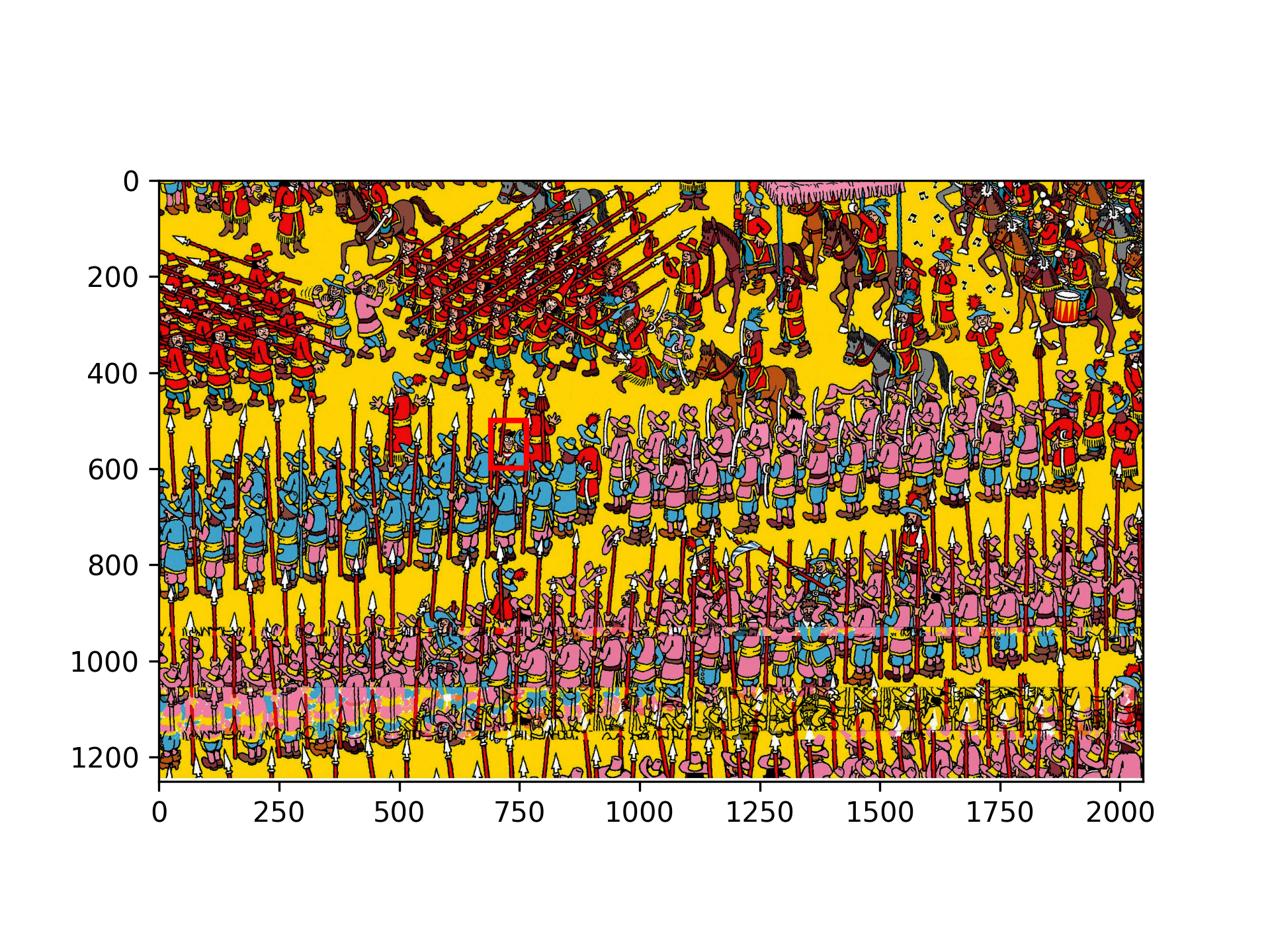
Fig. 15.18 Case_1_output.png

Case 2 Sample Output

$ python3 py5_ind_2_username.py Enter the path of the scene image you want to load: scene_2.jpg Enter the path of the template image you want to load: template_2.jpg The template is located at (1713, 401)

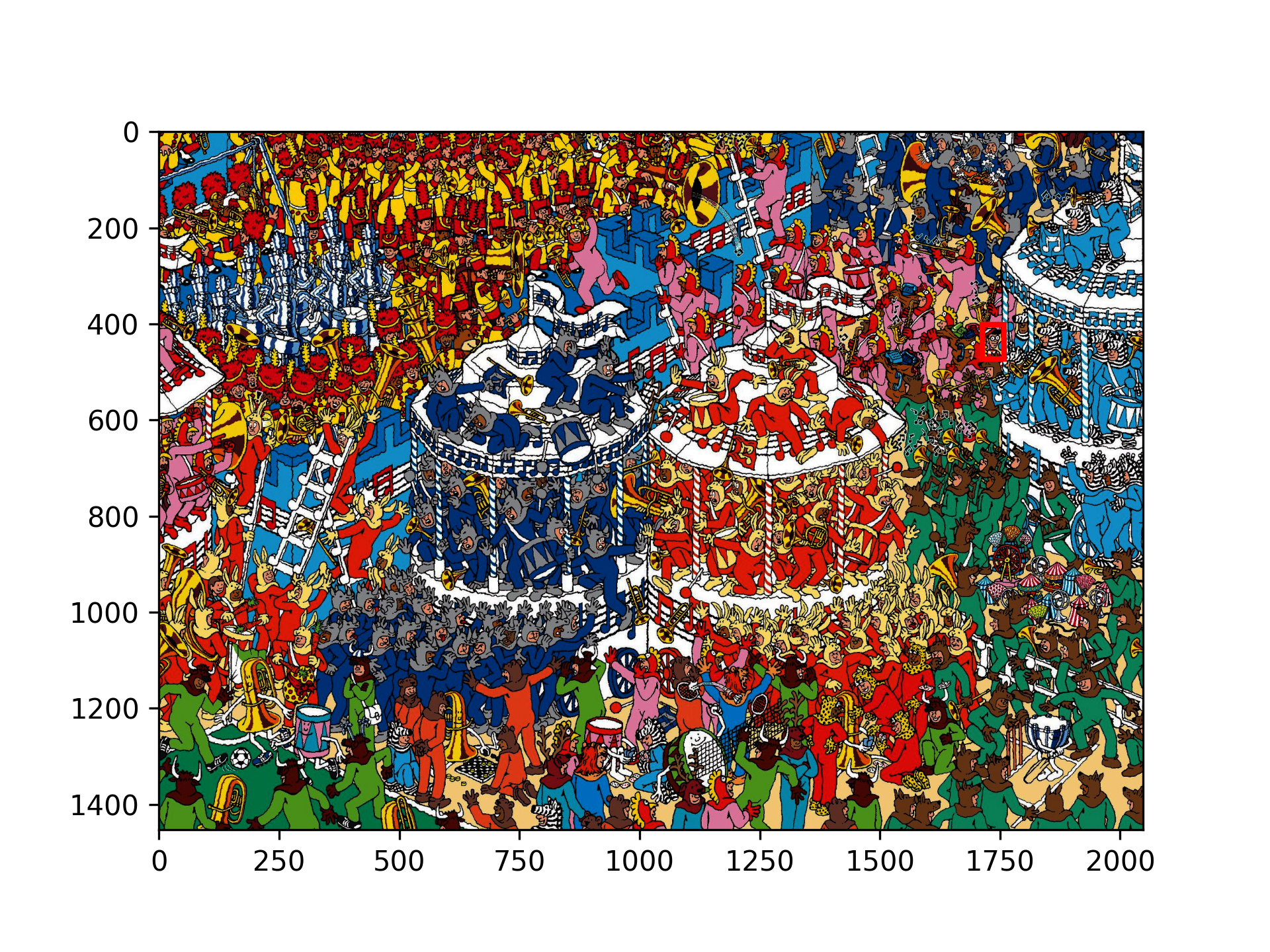
Fig. 15.19 Case_2_output.png

Case 3 Sample Output

$ python3 py5_ind_2_username.py Enter the path of the scene image you want to load: scene_3.jpg Enter the path of the template image you want to load: template_3.jpg The template is located at (1144, 285)

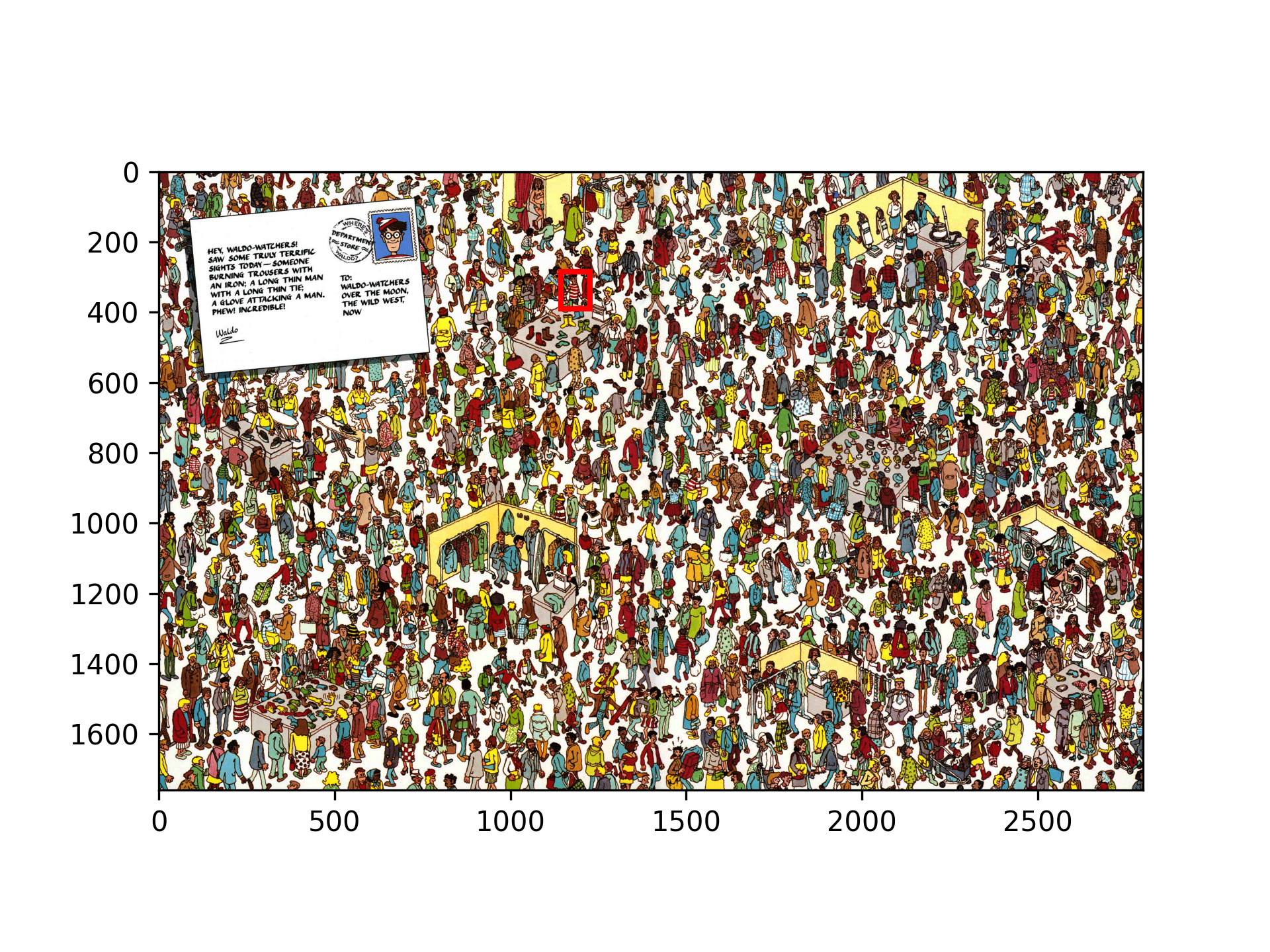
Fig. 15.20 Case_3_output.png

Table 15.16 Deliverables

Deliverables	Description
py5_ind_2_username.pdf	Flowchart(s) for this task.
py5_ind_2_username.py	Your completed Python code.