\[ \begin{align}\begin{aligned}\newcommand\blank{~\underline{\hspace{1.2cm}}~}\\% Bold symbols (vectors) \newcommand\bs[1]{\mathbf{#1}}\\% Differential \newcommand\dd[2][]{\mathrm{d}^{#1}{#2}} % use as \dd, \dd{x}, or \dd[2]{x}\\% Poor man's siunitx \newcommand\unit[1]{\mathrm{#1}} \newcommand\num[1]{#1} \newcommand\qty[2]{#1~\unit{#2}}\\\newcommand\per{/} \newcommand\squared{{}^2} \newcommand\cubed{{}^3} % % Scale \newcommand\milli{\unit{m}} \newcommand\centi{\unit{c}} \newcommand\kilo{\unit{k}} \newcommand\mega{\unit{M}} % % Percent \newcommand\percent{\unit{{\kern-4mu}\%}} % % Angle \newcommand\radian{\unit{rad}} \newcommand\degree{\unit{{\kern-4mu}^\circ}} % % Time \newcommand\second{\unit{s}} \newcommand\s{\second} \newcommand\minute{\unit{min}} \newcommand\hour{\unit{h}} % % Distance \newcommand\meter{\unit{m}} \newcommand\m{\meter} \newcommand\inch{\unit{in}} \newcommand\foot{\unit{ft}} % % Force \newcommand\newton{\unit{N}} \newcommand\kip{\unit{kip}} % kilopound in "freedom" units - edit made by Sri % % Mass \newcommand\gram{\unit{g}} \newcommand\g{\gram} \newcommand\kilogram{\unit{kg}} \newcommand\kg{\kilogram} \newcommand\grain{\unit{grain}} \newcommand\ounce{\unit{oz}} \newcommand\pound{\unit{lbs}} % % Temperature \newcommand\kelvin{\unit{K}} \newcommand\K{\kelvin} \newcommand\celsius{\unit{{\kern-4mu}^\circ C}} \newcommand\C{\celsius} \newcommand\fahrenheit{\unit{{\kern-4mu}^\circ F}} \newcommand\F{\fahrenheit} % % Area \newcommand\sqft{\unit{sq\,\foot}} % square foot % % Volume \newcommand\liter{\unit{L}} \newcommand\gallon{\unit{gal}} % % Frequency \newcommand\hertz{\unit{Hz}} \newcommand\rpm{\unit{rpm}} % % Voltage \newcommand\volt{\unit{V}} \newcommand\V{\volt} \newcommand\millivolt{\milli\volt} \newcommand\mV{\milli\volt} \newcommand\kilovolt{\kilo\volt} \newcommand\kV{\kilo\volt} % % Current \newcommand\ampere{\unit{A}} \newcommand\A{\ampere} \newcommand\milliampereA{\milli\ampere} \newcommand\mA{\milli\ampere} \newcommand\kiloampereA{\kilo\ampere} \newcommand\kA{\kilo\ampere} % % Resistance \newcommand\ohm{\Omega} \newcommand\milliohm{\milli\ohm} \newcommand\kiloohm{\kilo\ohm} % correct SI spelling \newcommand\kilohm{\kilo\ohm} % "American" spelling used in siunitx \newcommand\megaohm{\mega\ohm} % correct SI spelling \newcommand\megohm{\mega\ohm} % "American" spelling used in siunitx % % Capacitance \newcommand\farad{\unit{F}} \newcommand\F{\farad} \newcommand\microfarad{\micro\farad} \newcommand\muF{\micro\farad} % % Inductance \newcommand\henry{\unit{H}} \newcommand\H{\henry} \newcommand\millihenry{\milli\henry} \newcommand\mH{\milli\henry} % % Power \newcommand\watt{\unit{W}} \newcommand\W{\watt} \newcommand\milliwatt{\milli\watt} \newcommand\mW{\milli\watt} \newcommand\kilowatt{\kilo\watt} \newcommand\kW{\kilo\watt} % % Energy \newcommand\joule{\unit{J}} \newcommand\J{\joule} % % Composite units % % Torque \newcommand\ozin{\unit{\ounce}\,\unit{in}} \newcommand\newtonmeter{\unit{\newton\,\meter}} % % Pressure \newcommand\psf{\unit{psf}} % pounds per square foot \newcommand\pcf{\unit{pcf}} % pounds per cubic foot \newcommand\pascal{\unit{Pa}} \newcommand\Pa{\pascal} \newcommand\ksi{\unit{ksi}} % kilopound per square inch \newcommand\bar{\unit{bar}} \end{aligned}\end{align} \]

Apr 28, 2026 | 1296 words | 13 min read

14.3.2. Task 2

Learning Objectives:

• Reuse previously written functions to analyze new data.

• Load and interpret saved model data from CSV files.

• Compare frequency models using a quantitative distance metric.

• Visualize analysis results using plots.

Introduction

In Section 14.3.1 you built normalized n-gram frequency models for several known languages and saved them to CSV files. These models describe how frequently different character patterns appear in each language.

In this task, you will apply those models to analyze text files in an unknown language. Rather than simply choosing the closest match for a single n-gram size, you will examine how the model comparisons behave across multiple values of \(n\).

In this task, you will build n-gram models for the unknown language texts, compare those models to the known language models, and analyze the separation between the languages as you vary the n-gram size. This will allow you to reason not only about which language the unknown text is most likely written in, but also about which n-gram sizes are more effective than others for distinguishing between languages.

Task Instructions

Make sure you have successfully completed Section 14.3.1 and have the CSV files containing the n-gram models for each known language. You will need to read these files in this task.

Before creating the program, create a flowchart of the algorithm you will use and save it as py4_ind_2_username.pdf. Then start your program from a copy of the ENGR133_Python_Template.py Python template. Your program should be named py4_ind_2_username.py. You will also need to create a folder named unknown_texts within the same folder as your Python script. Then, download each of the unknown texts in Table 14.10 and place them into your unknown_texts folder. Develop a Python program that does the following:

1. Create relative frequency n-grams for each unknown text file.

2. Load the models from the CSV files created in Section 14.3.1.

3. For each unknown text, compute the distance between its n-gram model and each of the known language models for \(n\) from \(1\) to \(5\).

4. Calculate the separation scores for each of the n-gram sizes and find the best n-gram language model match for each unknown text based on these separation scores.

5. Generate a plot for each unknown text showing the separation scores for each known language across the different n-gram sizes.

Table 14.10 Unknown Text Download

Unknown Text	Download Link
Unknown Text 1	sample_unknown_1.txt
Unknown Text 2	sample_unknown_2.txt
Unknown Text 3	sample_unknown_3.txt

Note

Make sure you saved the samples into your unknown_texts folder, and that your folder is located in the same directory as your Python script.

Create Models Function

Create a function named create_models that has no parameters and returns a dictionary where the keys are the unknown file names (e.g., “unknown_1”, “unknown_2”) and the values are the corresponding relative frequency n-gram dictionaries.

The relative frequency n-gram dictionaries should be structured such that each key is an n-gram size (from \(1\) to \(5\)), and each value is another dictionary where the keys are the n-grams and the values are the relative frequencies of those n-grams in the unknown text.

This function should replicate the process you used in the previous task to create relative frequency n-gram models for the known languages, but it should be applied to the unknown text files instead. It is STRONGLY ADVISED to reuse the load_samples, clean_text, create_n_gram, and normalize_n_gram functions that you created in Section 14.3.1 to help with this process.

Load From CSV Function

Create a function named load_from_csv that has no parameters and returns a dictionary where the keys are the known languages (e.g., “english”, “french”) and the values are the corresponding relative frequency n-gram dictionaries.

When reading the CSV files, ensure that you correctly parse the n-grams and their relative frequencies for each n-gram size from the CSV files. Pay very close attention to the structure you used when saving the models in Section 14.3.1, as you will need to read the data back in the same format. You can use the csv module from the Python standard library to help with this task, reference the official documentation for more information.

N-Gram Distance Function

Create a function named n_gram_dist that takes in two n-gram dictionaries of the same n (one for the unknown text and one for a known language) and returns the total distance between the two n-gram models using a distance metric. The keys for the n-gram dictionaries will be the n-grams and the values will be the relative frequencies of those n-grams.

The distance metric you will implement is the absolute difference between the relative frequencies of the n-grams in the two models. To calculate this, you will need to iterate through all n-grams that appear in either model and use the following formula:

(14.2)\[\begin{split}\text{Distance} = \begin{cases} |L-U|\text{ if n-gram is in both models}\\ L\text{ if n-gram is only in language model}\\ U\text{ if n-gram is only in unknown model} \end{cases}\end{split}\]

Where \(L\) is the relative frequency of the n-gram in the known language model and \(U\) is the relative frequency of the n-gram in the unknown language model.

By summing the distances for all n-grams, you will get a total distance score that quantifies how different the two models are. A smaller distance indicates that the unknown text is more similar to the known language, while a larger distance indicates that it is less similar.

Score Language Function

Create a function named score_language that takes a dictionary of known language n-gram models (as returned by the load_from_csv function), a dictionary of a single unknown text n-gram (the keys will be n-grams and the values will be the relative frequencies of those n-grams), and the desired n-gram size n. This function will return a dictionary whose keys are the known language names and values are the total distance scores for each known language model compared to the unknown text model for the specified n-gram size.

Use the n_gram_dist function to calculate the distance between the unknown text model and each known language model for the specified n-gram size.

Score Separation Function

Create a function named score_separation that takes in a dictionary of distance scores for each known language (as returned by the score_language function) and returns a dictionary whose keys are the known language names and values are the separation score for that language.

The separation score is a way of measuring how much a particular distance score stands out from the others. Here we are just finding the average difference in distance scores between a particular language and all the other languages. The formula for calculating the separation score for a single language is as follows:

(14.3)\[\text{Separation Score} = \frac{\sum_{i=1}^{n} |x_i - \overline{x}|}{n - 1}\]

Where:

• \(x_i\) is each distance score for a language

• \(\overline{x}\) is the distance score for the language being evaluated

• \(n\) is the number of known languages

You can think of the separation score as a measure of how much a particular language’s distance score stands out from the others. A higher separation score indicates that the language is more distinct from the others, while a lower separation score indicates that it is more similar to the others.

Plotting Function

Create a function named plot_separation_vs_n that takes in a dictionary of separation scores for each known language across different n-gram sizes (the keys will be n-gram sizes and the values will be language separation score dictionaries as returned by the score_separation function) and the name of the unknown text. This function should generate a plot showing how the separation scores for each known language change as the n-gram size varies. This function template is provided for you. You will need to fill in the TODO sections to complete the function.

import matplotlib.pyplot as plt

def plot_separation_vs_n(scores_by_n, name):
    fig, axs = plt.subplots(2, 3, figsize=(15, 10), sharey=True)

    n_values = sorted([int(n) for n in scores_by_n.keys()])

    # languages from the first n entry (assumes all n have same languages)
    first_n = str(n_values[0])
    languages = sorted(scores_by_n[first_n].keys())

    row = 0
    col = 0

    for language in languages:
        ax = axs[row][col]

        # collect y-values (scores) in order of n
        y_scores = []
        for n in n_values:
            y_scores.append(scores_by_n[str(n)][language])

        # TODO :
        # Set the x and y labels, title, and plot the points

        ax.set_xticks(n_values)

        col += 1
        if col == 3:
            col = 0
            row += 1

    plt.suptitle(f"{name} Language Separation", fontsize=16)
    plt.tight_layout()
    plt.show()

Main Function

In your main function, you will need to do the following:

1. Create the unknown language n-gram models using the create_models function.

2. Load the known language n-gram models using the load_from_csv function.

3. Display the unknown texts in the unknown_texts folder, and have the user select a text to analyze.

4. For the selected unknown text, iterate through all n values (\(1\) through \(5\)) and get the language scores and separation scores.

5. Print the best n-gram language model match for the unknown text.

6. Plot the n separation values for the unknown text.

Sample Output

Test cases for language identification and visualization. Use the values in Table 14.11 below to test your program.

Table 14.11 Test Cases

Case	Unknown Filename
1	unknown_1
2	unknown_2
3	unknown_3

Ensure your program’s output matches the provided samples exactly. This includes all characters, white space, and punctuation. In the samples, user input is highlighted like this for clarity, but your program should not highlight user input in this way.

Case 1 Sample Output

$ python3 py4_ind_2_username.py Unknown Language File Options 1. unknown_3 2. unknown_2 3. unknown_1 Select a file to analyze: unknown_1 The best language match for unknown_1 is the 4-gram english model.

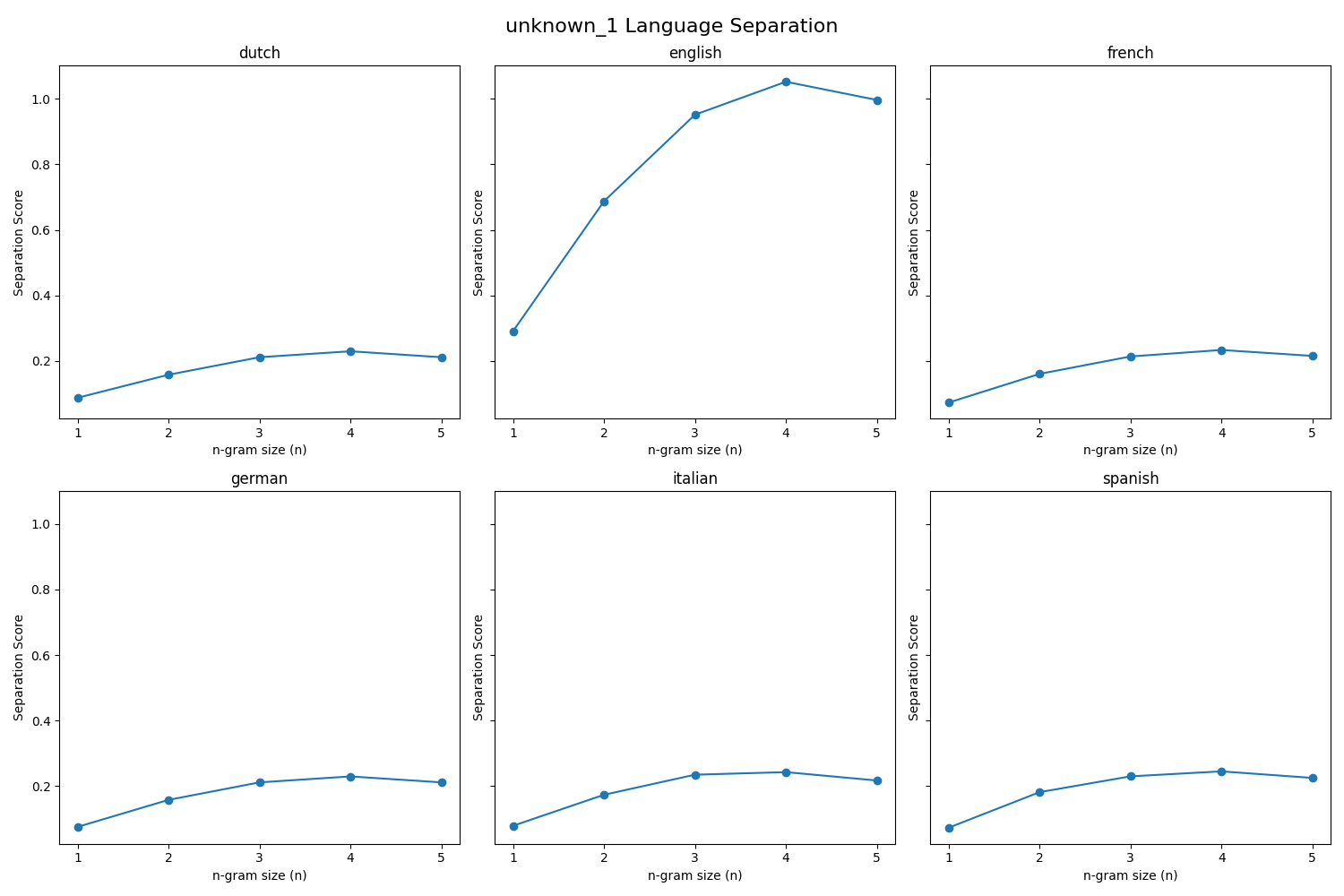
Fig. 14.5 Case_1_output.png

Case 2 Sample Output

$ python3 py4_ind_2_username.py Unknown Language File Options 1. unknown_3 2. unknown_2 3. unknown_1 Select a file to analyze: unknown_2 The best language match for unknown_2 is the 4-gram french model.

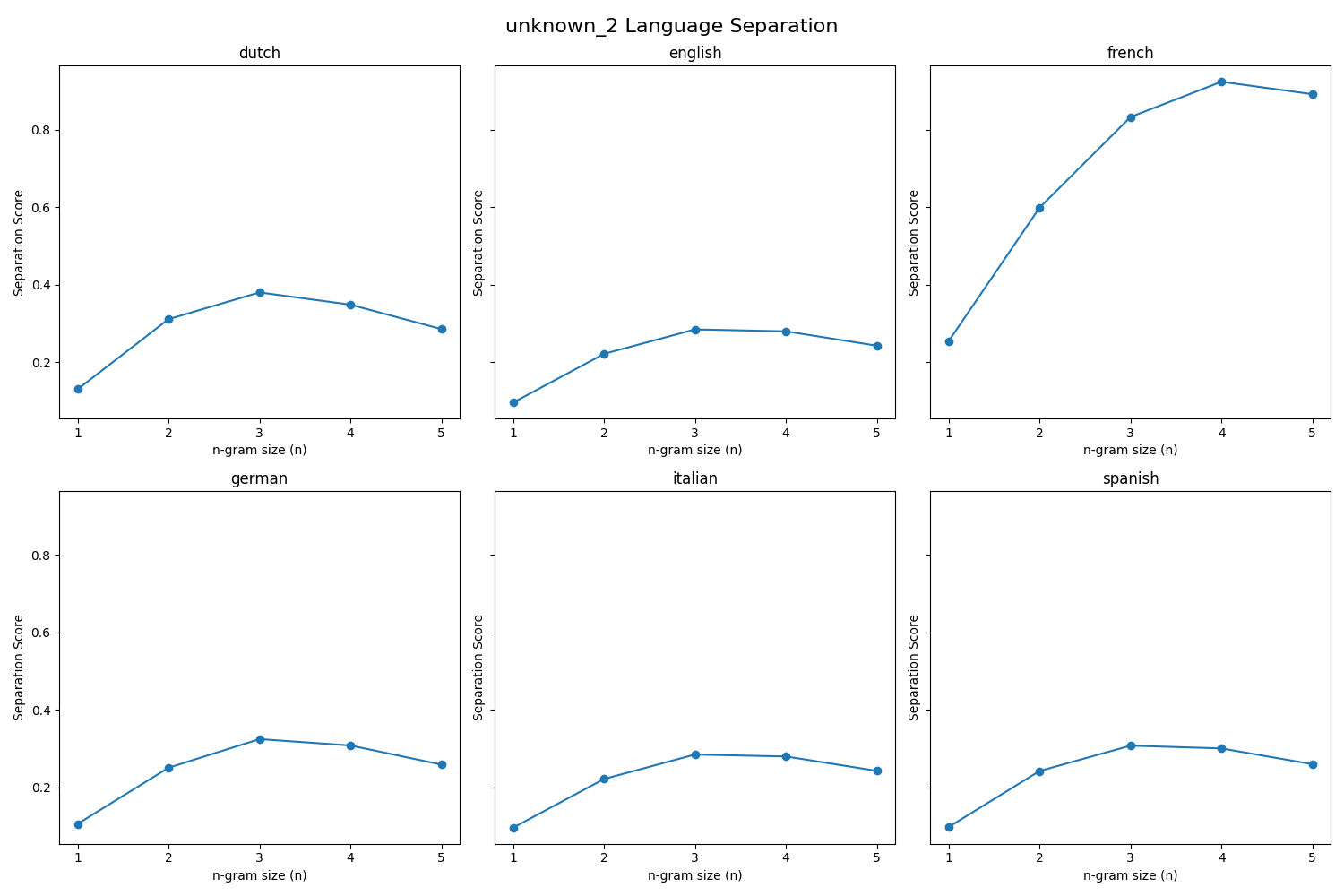
Fig. 14.6 Case_2_output.png

Case 3 Sample Output

$ python3 py4_ind_2_username.py Unknown Language File Options 1. unknown_3 2. unknown_2 3. unknown_1 Select a file to analyze: unknown_3 The best language match for unknown_3 is the 4-gram italian model.

Fig. 14.7 Case_3_output.png

Table 14.12 Deliverables

Deliverables	Description
py4_ind_2_username.pdf	Flowchart(s) for this task.
py4_ind_2_username.py	Your completed Python code.