\[ \begin{align}\begin{aligned}\newcommand\blank{~\underline{\hspace{1.2cm}}~}\\% Bold symbols (vectors) \newcommand\bs[1]{\mathbf{#1}}\\% Differential \newcommand\dd[2][]{\mathrm{d}^{#1}{#2}} % use as \dd, \dd{x}, or \dd[2]{x}\\% Poor man's siunitx \newcommand\unit[1]{\mathrm{#1}} \newcommand\num[1]{#1} \newcommand\qty[2]{#1~\unit{#2}}\\\newcommand\per{/} \newcommand\squared{{}^2} \newcommand\cubed{{}^3} % % Scale \newcommand\milli{\unit{m}} \newcommand\centi{\unit{c}} \newcommand\kilo{\unit{k}} \newcommand\mega{\unit{M}} % % Percent \newcommand\percent{\unit{{\kern-4mu}\%}} % % Angle \newcommand\radian{\unit{rad}} \newcommand\degree{\unit{{\kern-4mu}^\circ}} % % Time \newcommand\second{\unit{s}} \newcommand\s{\second} \newcommand\minute{\unit{min}} \newcommand\hour{\unit{h}} % % Distance \newcommand\meter{\unit{m}} \newcommand\m{\meter} \newcommand\inch{\unit{in}} \newcommand\foot{\unit{ft}} % % Force \newcommand\newton{\unit{N}} \newcommand\kip{\unit{kip}} % kilopound in "freedom" units - edit made by Sri % % Mass \newcommand\gram{\unit{g}} \newcommand\g{\gram} \newcommand\kilogram{\unit{kg}} \newcommand\kg{\kilogram} \newcommand\grain{\unit{grain}} \newcommand\ounce{\unit{oz}} \newcommand\pound{\unit{lbs}} % % Temperature \newcommand\kelvin{\unit{K}} \newcommand\K{\kelvin} \newcommand\celsius{\unit{{\kern-4mu}^\circ C}} \newcommand\C{\celsius} \newcommand\fahrenheit{\unit{{\kern-4mu}^\circ F}} \newcommand\F{\fahrenheit} % % Area \newcommand\sqft{\unit{sq\,\foot}} % square foot % % Volume \newcommand\liter{\unit{L}} \newcommand\gallon{\unit{gal}} % % Frequency \newcommand\hertz{\unit{Hz}} \newcommand\rpm{\unit{rpm}} % % Voltage \newcommand\volt{\unit{V}} \newcommand\V{\volt} \newcommand\millivolt{\milli\volt} \newcommand\mV{\milli\volt} \newcommand\kilovolt{\kilo\volt} \newcommand\kV{\kilo\volt} % % Current \newcommand\ampere{\unit{A}} \newcommand\A{\ampere} \newcommand\milliampereA{\milli\ampere} \newcommand\mA{\milli\ampere} \newcommand\kiloampereA{\kilo\ampere} \newcommand\kA{\kilo\ampere} % % Resistance \newcommand\ohm{\Omega} \newcommand\milliohm{\milli\ohm} \newcommand\kiloohm{\kilo\ohm} % correct SI spelling \newcommand\kilohm{\kilo\ohm} % "American" spelling used in siunitx \newcommand\megaohm{\mega\ohm} % correct SI spelling \newcommand\megohm{\mega\ohm} % "American" spelling used in siunitx % % Capacitance \newcommand\farad{\unit{F}} \newcommand\F{\farad} \newcommand\microfarad{\micro\farad} \newcommand\muF{\micro\farad} % % Inductance \newcommand\henry{\unit{H}} \newcommand\H{\henry} \newcommand\millihenry{\milli\henry} \newcommand\mH{\milli\henry} % % Power \newcommand\watt{\unit{W}} \newcommand\W{\watt} \newcommand\milliwatt{\milli\watt} \newcommand\mW{\milli\watt} \newcommand\kilowatt{\kilo\watt} \newcommand\kW{\kilo\watt} % % Energy \newcommand\joule{\unit{J}} \newcommand\J{\joule} % % Composite units % % Torque \newcommand\ozin{\unit{\ounce}\,\unit{in}} \newcommand\newtonmeter{\unit{\newton\,\meter}} % % Pressure \newcommand\psf{\unit{psf}} % pounds per square foot \newcommand\pcf{\unit{pcf}} % pounds per cubic foot \newcommand\pascal{\unit{Pa}} \newcommand\Pa{\pascal} \newcommand\ksi{\unit{ksi}} % kilopound per square inch \newcommand\bar{\unit{bar}} \end{aligned}\end{align} \]

Apr 28, 2026 | 931 words | 9 min read

15.3.1. Task 1

Learning Objectives

• Utilize the pathlib library to access and manage files in a directory.

• Manipulate matrices using NumPy.

• Utilize matplotlib functions to display data.

• Visualize the distribution of color intensities in an image.

Introduction

Digital image processing plays a vital role across many areas of engineering, from medical diagnostics to satellite imaging. A key task in this field is analyzing an image’s color distribution, which can be visualized with a histogram where the x-axis represents intensity values (\(0\)–\(255\) for 8-bit images) and the y-axis shows the frequency of each value. This visualization reveals an image’s brightness, contrast, and overall color balance, and provides insights that are essential for applications such as image enhancement, segmentation, and object detection.

An image’s overall brightness, or luminance, can be calculated using a weighted sum of its red, green, and blue channel values. The weights (\(0.2126\), \(0.7152\), and \(0.0722\)) are derived from the sRGB color space and reflect the human eye’s sensitivity to different wavelengths of light. You can read more about relative luminance on Wikipedia. The formula for luminance is given in (15.8).

Task Instructions

Develop a Python program that produces a color distribution histogram of a user selected image to aid in image analysis. The program should allow the user to select from a list of all images in their images folder.

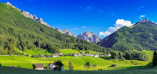
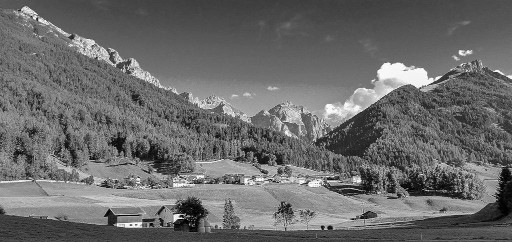
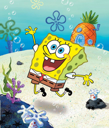
Before writing your program, create a flowchart of your algorithm and save it as py5_ind_1_username.pdf. Then, start coding by making a copy of the ENGR133_Python_Template.py Python template. Name your program py5_ind_1_username.py. You will also need to create a folder named images within the same folder as your Python script. Then, download each of the sample images in Table 15.11 and place them into your images folder. You can use your own images if you prefer, but ensure they are in a common format such as PNG or JPEG.

Table 15.11 Sample Images

Image	Download
	spongebob.jpg,
	landscape.jpeg
	grayscale_landscape.jpeg.

Note

Ensure that you have the correct folder open in VS Code to avoid errors. You can select your folder by opening VS Code, clicking File (at the top of your screen), clicking Open Folder…, and selecting your desired folder. Now when you open the Explorer pane you should see something similar to :

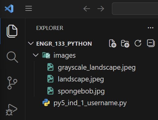
Fig. 15.13 Sample Folder Structure

Your program should do the following:

1. Construct a menu that lists all images in your images folder and allows the user to select one by entering its corresponding number. Be sure to include an option to quit the program.

   Hint

   The iterdir() method from Python’s pathlib module can be used to create a list all files in a directory. Your output is allowed to have the files displayed in a different order than the sample output.

   from pathlib import Path
   
   path = Path('images')
   files = list(path.iterdir())
   

   Hint

   You will need to find a way to exclude non-image files from your menu. Path objects have a suffix method that may be useful for this. You can read more about it in the official documentation.

2. Load the selected image, verify the image’s data type, and normalize the pixel values.

3. Linearize the pixels in the image array.

4. Calculate the average luminance of the image and display the result in the terminal.

5. Plot the distribution of pixel intensity for the linearized image array.

Load Image Function

Create a function named load_image that takes in the path of the image as a string and returns a normalized np.array representing the image data.

Use Image.open(path) from the PIL module to load the image. Then convert the resulting Image object into a NumPy array. Verify that the data type of your NumPy array is numpy.uint8, which will have pixel values in the range \([0, 255]\). If the image has any other data type, raise a ValueError with the message “Image is not 8-bit.” Reference Section 13.1.1 for more details about how to check this. Finally, normalize the pixel values in the NumPy array to the range \([0.0, 1.0]\).

Calculate Luminance Function

Create a function named calculate_luminance that takes in an np.array of linearized pixel values and returns the average luminance of the entire image array.

The luminance of a pixel is calculated using the following formula:

(15.8)\[Y = 0.2126 \cdot R + 0.7152 \cdot G + 0.0722 \cdot B\]

where \(R\), \(G\), and \(B\) are the linearized values of the red, green, and blue channels, respectively.

Plotting Function

Create a function named plot_pixel_intensity with an np.array of linearized pixel values as its argument.

Create a figure with two side-by-side subplots using matplotlib. Show the linearized image on the left, and on the right, plot an intensity histogram showing the distribution of pixel values for each channel (red, green, and blue for color images, or gray for grayscale images).

Note

For color images, plot three overlapping histograms (one for each channel) using the colors red, green, and blue. Use an alpha value of \(0.5\) to make the histograms semi-transparent so that overlapping areas can be seen. You will need to find a way to convert each channel’s values from a 2-dimensional array to a 1-dimensional array. Then the code to add the histogram for each channel to the plot should look something like this:

axes[1].hist(channel_values, bins=256, color='red', alpha=0.5)

Main Function

In your main function, you will need to do the following:

1. Provide the menu of available images and prompt the user to select an image or quit the program.

2. Quit the program if selected.

3. Otherwise, load, verify the data type, and normalize the selected image using the load_image function.

4. Linearize the pixel values in the image array.

5. Calculate the average luminance using the calculate_luminance function and display the result.

6. Plot the distribution of pixel intensity in the linearized array using the plot_pixel_intensity function.

7. Repeat.

Sample Output

Use the values in Table 15.12 below to test your program.

Table 15.12 Test Cases

Case	User Input
1	[1, ‘q’]
2	[‘spam’, 2, ‘q’]
3	[3, ‘q’]

Ensure your program’s output matches the provided samples exactly. This includes all characters, white space, and punctuation. In the samples, user input is highlighted like this for clarity, but your program should not highlight user input in this way.

Case 1 Sample Output

$ python3 py5_ind_1_username.py Available images: 1. spongebob.jpg 2. grayscale_landscape.jpeg 3. landscape.jpeg Select an image (q to quit): 1 The average luminance of the image: 0.553

Available images: 1. spongebob.jpg 2. grayscale_landscape.jpeg 3. landscape.jpeg Select an image (q to quit): q

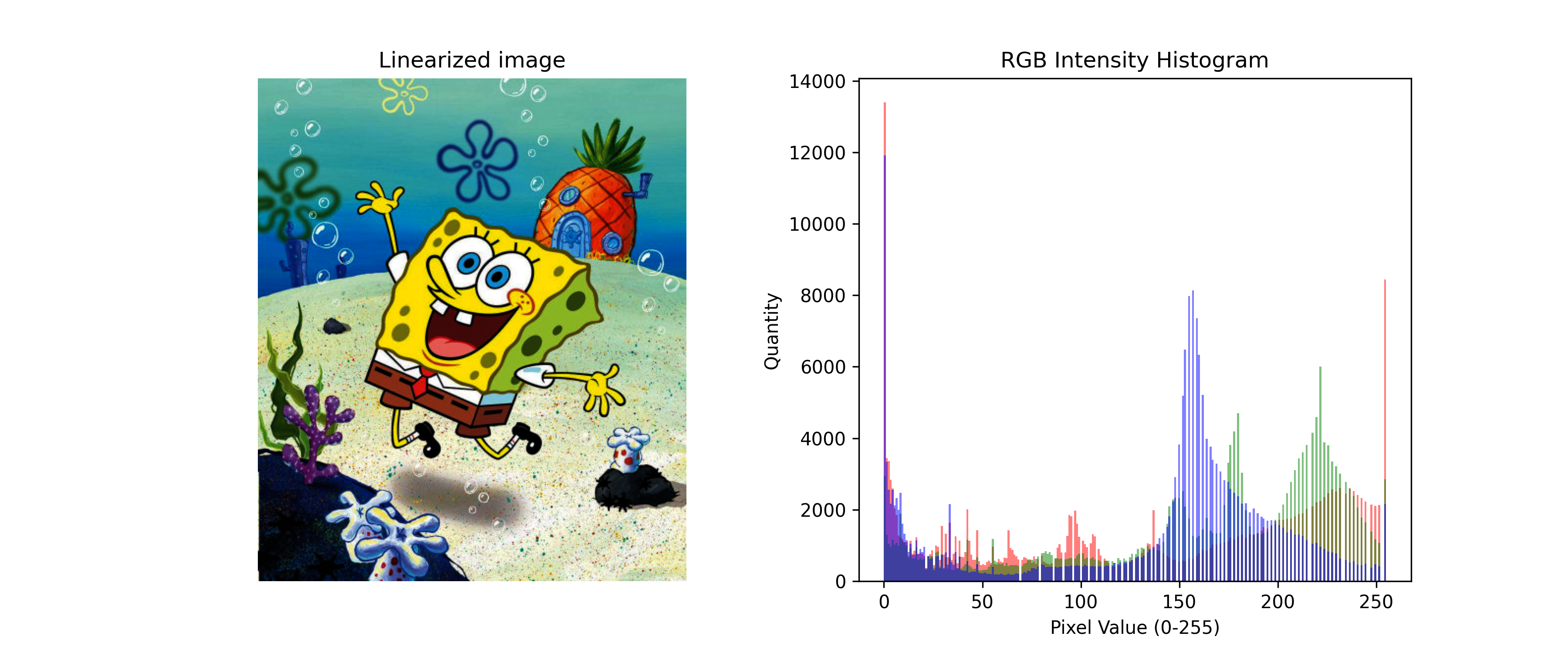
Fig. 15.14 Case_1_output.png

Case 2 Sample Output

$ python3 py5_ind_1_username.py Available images: 1. spongebob.jpg 2. grayscale_landscape.jpeg 3. landscape.jpeg Select an image (q to quit): spam Invalid choice, please try again.

Available images: 1. spongebob.jpg 2. grayscale_landscape.jpeg 3. landscape.jpeg Select an image (q to quit): 2 The average luminance of the image: 0.178

Available images: 1. spongebob.jpg 2. grayscale_landscape.jpeg 3. landscape.jpeg Select an image (q to quit): q

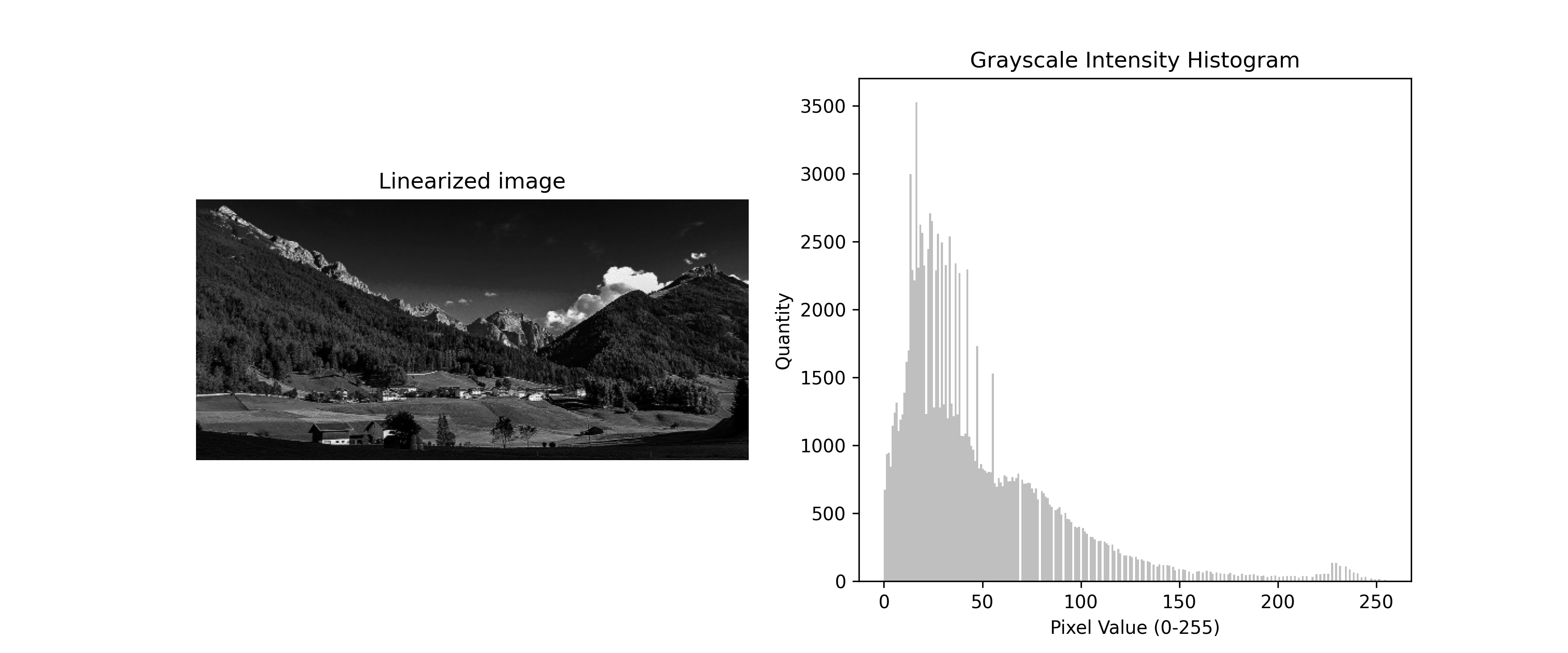
Fig. 15.15 Case_2_output.png

Case 3 Sample Output

$ python3 py5_ind_1_username.py Available images: 1. spongebob.jpg 2. grayscale_landscape.jpeg 3. landscape.jpeg Select an image (q to quit): 3 The average luminance of the image: 0.210

Available images: 1. spongebob.jpg 2. grayscale_landscape.jpeg 3. landscape.jpeg Select an image (q to quit): q

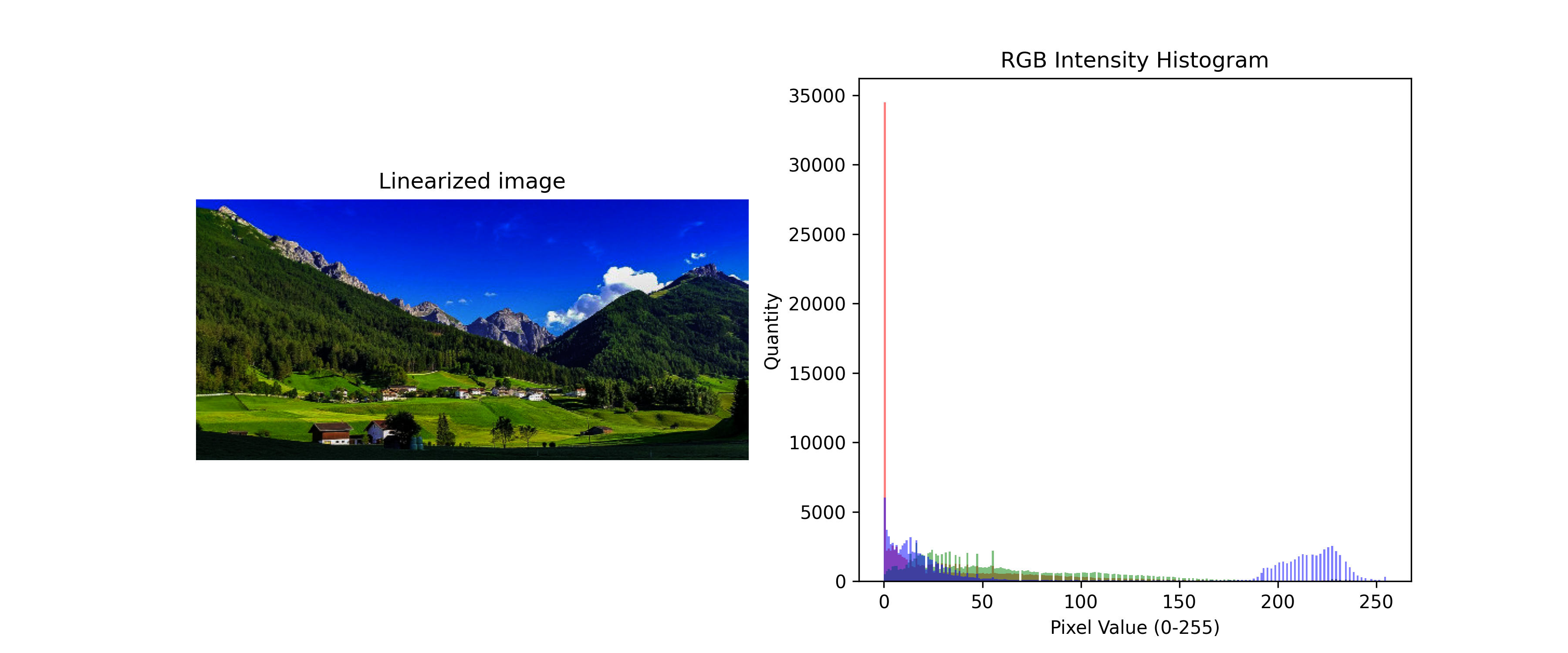
Fig. 15.16 Case_3_output.png

Table 15.13 Deliverables

Deliverables	Description
py5_ind_1_username.py	Your completed Python code.
py5_ind_1_username.pdf	Flowchart(s) for this task.