\[ \begin{align}\begin{aligned}\newcommand\blank{~\underline{\hspace{1.2cm}}~}\\% Bold symbols (vectors) \newcommand\bs[1]{\mathbf{#1}}\\% Poor man's siunitx \newcommand\unit[1]{\mathrm{#1}} \newcommand\num[1]{#1} \newcommand\qty[2]{#1~\unit{#2}}\\\newcommand\per{/} \newcommand\squared{{}^2} \newcommand\cubed{{}^3} % % Scale \newcommand\milli{\unit{m}} \newcommand\centi{\unit{c}} \newcommand\kilo{\unit{k}} \newcommand\mega{\unit{M}} % % Percent \newcommand\percent{\unit{\%}} % % Angle \newcommand\radian{\unit{rad}} \newcommand\degree{\unit{{}^\circ}} % % Time \newcommand\second{\unit{s}} \newcommand\s{\second} \newcommand\minute{\unit{min}} \newcommand\hour{\unit{h}} % % Distance \newcommand\meter{\unit{m}} \newcommand\m{\meter} \newcommand\inch{\unit{in}} \newcommand\foot{\unit{ft}} % % Force \newcommand\newton{\unit{N}} \newcommand\kip{\unit{kip}} % kilopound in "freedom" units - edit made by Sri % % Mass \newcommand\gram{\unit{g}} \newcommand\g{\gram} \newcommand\kilogram{\unit{kg}} \newcommand\kg{\kilogram} \newcommand\grain{\unit{grain}} \newcommand\ounce{\unit{oz}} % % Temperature \newcommand\kelvin{\unit{K}} \newcommand\K{\kelvin} \newcommand\celsius{\unit{{}^\circ C}} \newcommand\C{\celsius} \newcommand\fahrenheit{\unit{{}^\circ F}} \newcommand\F{\fahrenheit} % % Area \newcommand\sqft{\unit{sq\,\foot}} % square foot % % Volume \newcommand\liter{\unit{L}} \newcommand\gallon{\unit{gal}} % % Frequency \newcommand\hertz{\unit{Hz}} \newcommand\rpm{\unit{rpm}} % % Voltage \newcommand\volt{\unit{V}} \newcommand\V{\volt} \newcommand\millivolt{\milli\volt} \newcommand\mV{\milli\volt} \newcommand\kilovolt{\kilo\volt} \newcommand\kV{\kilo\volt} % % Current \newcommand\ampere{\unit{A}} \newcommand\A{\ampere} \newcommand\milliampereA{\milli\ampere} \newcommand\mA{\milli\ampere} \newcommand\kiloampereA{\kilo\ampere} \newcommand\kA{\kilo\ampere} % % Resistance \newcommand\ohm{\Omega} \newcommand\milliohm{\milli\ohm} \newcommand\kiloohm{\kilo\ohm} % correct SI spelling \newcommand\kilohm{\kilo\ohm} % "American" spelling used in siunitx \newcommand\megaohm{\mega\ohm} % correct SI spelling \newcommand\megohm{\mega\ohm} % "American" spelling used in siunitx % % Inductance \newcommand\henry{\unit{H}} \newcommand\H{\henry} \newcommand\millihenry{\milli\henry} \newcommand\mH{\milli\henry} % % Power \newcommand\watt{\unit{W}} \newcommand\W{\watt} \newcommand\milliwatt{\milli\watt} \newcommand\mW{\milli\watt} \newcommand\kilowatt{\kilo\watt} \newcommand\kW{\kilo\watt} % % Energy \newcommand\joule{\unit{J}} \newcommand\J{\joule} % % Composite units % % Torque \newcommand\ozin{\unit{\ounce}\,\unit{in}} \newcommand\newtonmeter{\unit{\newton\,\meter}} % % Pressure \newcommand\psf{\unit{psf}} % pounds per square foot \newcommand\pcf{\unit{pcf}} % pounds per cubic foot \newcommand\pascal{\unit{Pa}} \newcommand\Pa{\pascal} \newcommand\ksi{\unit{ksi}} % kilopound per square inch \newcommand\bar{\unit{bar}} \end{aligned}\end{align} \]

Oct 24, 2024 | 1095 words | 11 min read

8.3.1. Task 1

Image Analysis

Learning Objectives:

• Utilize file I/O functions in Python to handle image data using modern Python libraries.

• Analyze image properties such as color composition and brightness using manual looping methods.

• Develop an understanding of Python libraries for image processing.

• Generate visual representations of image analysis results through histograms.

Introduction

Digital images form a critical part of daily digital media interaction, ranging from personal photography to professional graphics. Analyzing these images can unveil insights into color trends and image composition, thus deepening our understanding of visual preferences in digital content. This project uses Python’s robust libraries to dissect the color content and brightness of images, providing a hands-on approach to digital media analysis through computational methods.

Task Instructions

Develop a Python program named that performs analysis on a collection of images to primarily determine color content with a focus on red and evaluate the brightness of each image. The program will present insights through numerical data and visual histograms.

Luminosity Formula

Color Luminance and Contrast Ratio

The luminosity formula is a method used to convert a color image to grayscale by taking into account the different contributions of each color (red, green, and blue) to human perception of brightness. It is based on the human visual system’s differing sensitivity to various colors. The formula assigns weights to the red, green, and blue components of each pixel according to these sensitivities:

• Red: 0.299

• Green: 0.587

• Blue: 0.114

These values represent the perceived luminance of typical human vision for each color, ensuring that the resulting grayscale image accurately reflects the true perceived brightness.

Steps:

1. Read and load images:

   • Load images from a specified directory using pathlib, supporting common formats like PNG and JPEG.

2. Color Analysis:

   • Calculate the content of red color in each image.

3. Brightness Analysis:

   • Manually calculate the average brightness of each image by iterating over each pixel.

4. Output Analysis Results:

   • Write the analysis results, including red content and brightness, into a text file.

5. Visualization:

   • Generate histograms showing the distribution of color intensities, focusing on total and each colors specifically, without using advanced numpy functions like .ravel().

   • Refer to student_output.py file for example usage in histograms for the total intensity.

Functions

The program will incorporate the following key functions to handle various aspects of image analysis. Each function is designed to be modular and reusable, facilitating ease of maintenance and potential extension:

1. load_images(directory):

   • Purpose: Loads all images from a specified directory using pathlib for enhanced path handling.

   • Inputs: A string representing the directory path.

   • Outputs: A list of tuples, each containing an image loaded into a numpy array and its filename.

2. analyze_red_content(image):

   • Purpose: Analyzes the red color content in an image by computing the mean intensity of the red channel.

   • Explanation: The red channel can be accessed using image[:, :, 0]. This indexing selects all rows and columns in the first layer of the 3D array which corresponds to the red channel of the image.

   • Inputs: An image as a numpy array.

   • Outputs: A float representing the mean intensity of the red channel.

3. calculate_brightness(image):

   • Purpose: Calculates the average brightness of an image using the luminosity method, iterating over each pixel to manually compute the brightness without using numpy’s average function.

   • Explanation: Each pixel’s red, green, and blue values are accessed by iterating through the array’s dimensions. The luminosity formula is then manually applied to these values to calculate a grayscale value that reflects human visual sensitivity to these colors.

   • Inputs: An image as a numpy array.

   • Outputs: A float representing the average brightness of the image, calculated through manual summation and division.

4. write_results(filename, images):

   • Purpose: Writes the analysis results, including red content and brightness, to a specified text file.

   • Inputs: A string for the filename and a list of image data.

   • Outputs: None. Results are written directly to a file on disk.

5. generate_visualizations(images):

   • Purpose: Generates histograms for visual representation of color distributions within each image using manual histogram calculations.

   • Inputs: A list of images, each as a numpy array.

   • Explanation: This function leverages the plt.hist function for plotting histograms. For color images, separate histograms are plotted for each color channel to visually represent the distribution of pixel intensities. The .flatten() method is used to convert the multi-dimensional array of image data into a 1D array for histogram computation.

   • Outputs: None. Visualizations are displayed using matplotlib’s plotting functions, enhanced with manual histogram plotting to provide a deep learning experience about the histogram creation process.

   • Code Snippet: The code snippet below demonstrates how to generate histograms for both grayscale and color images. Implement the histogram plotting for the red, green, and blue channels in the indicated section.

   def generate_visualizations(images):
    for image, name in images:
        plt.figure()  # Create a new figure
   
        if image.ndim == 2:  # Check if the image is grayscale
            # Plot histogram for grayscale image
            plt.hist(image.flatten(), bins=256, color='gray', alpha=0.7, label='Intensity')
            plt.title(f'Intensity Histogram - {name}')  # Set the title of the histogram
   
        elif image.ndim == 3:  # Check if the image is color
            # Plot histograms for each color channel and the total intensity
            plt.hist(image.flatten(), bins=256, color='orange', alpha=0.5, label='Total')
            ### Start of your code
   
   
   
            ### End of your code
            plt.title(f'Color Histogram - {name}')  # Set the title of the histogram
        plt.xlabel('Intensity')  # Label the x-axis
        plt.ylabel('Frequency')  # Label the y-axis
        plt.legend()  # Display the legend
        plt.savefig('Histogram.png')  # Show the plot
   

These functions collaborate to process image data efficiently, providing insights into the color and brightness characteristics of each image in the dataset. By focusing on specific colors (such as red) and general image brightness through manual calculations, the program offers a comprehensive approach to image analysis suitable for educational purposes in data science and digital media.

Hints on Luminosity

• image[i, j, 0] Accesses the red channel of the pixel located at row i and column j. In a color image, image[i, j] would contain three values, corresponding to the red, green, and blue channels, with [0] specifically selecting the red channel.

• \(0.299\): This multiplier applies the weight assigned to the red channel as part of the luminosity formula. The value is derived from human vision research that determined how sensitive our eyes are to red light relative to other colors.

image[i, j, 0] * 0.299

Hints on Path

• Convert a directory string into a Path object: This provides a convenient way to handle file paths and directories using methods and attributes tailored for path manipulations.

• Using the .iterdir() method, you can iterate over files and directories in the given path. This makes it easy to check file extensions and process each file individually.

• The .name and .suffix attributes of a Path can be used to access the filename and extension from a path, respectively.

directory_path = Path(directory)  # Convert the directory string to a Path object

for img_path in directory_path.iterdir(): # Use Path.iterdir() to loop over all files in the directory

Hints on Handling Multi-dimensional array

The .flatten() method creates a one-dimensional array from any multi-dimensional array. When working with images represented as NumPy arrays, .flatten() converts the data into a single array that lists all pixel values sequentially.

This is useful when:

• Plotting histograms: Flattening an image simplifies counting pixel intensities, as histograms generally require a one-dimensional input.

• Simplifying analysis: A flattened array is easier to iterate over and apply mathematical operations to, compared to a multi-dimensional array.

flattened_data = image.flatten()

Table 8.5 Image Download

Images	Download Link
RGB image	rgb_image.jpeg
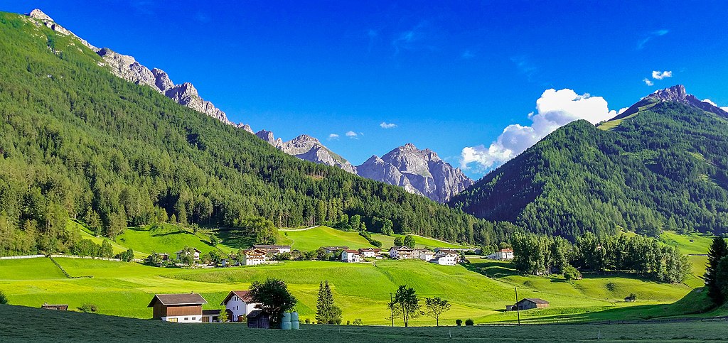
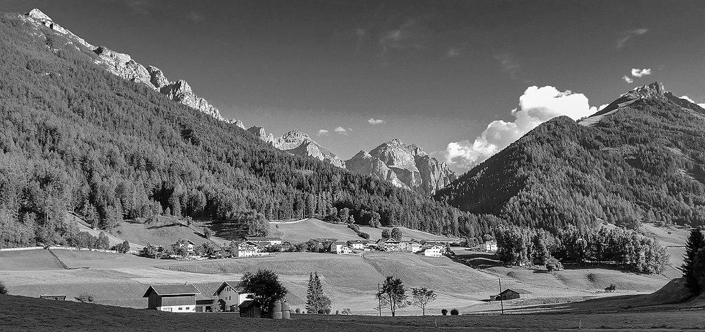
Grayscale image	grayscale_image.jpeg

Sample Output

Test cases for the image processing and histogram generation. Use the values in Table 8.6 below to test your program.

Table 8.6 Test Cases

Case	image directory
1	images
2	grayscale_images
3	empty_images

Ensure your program’s output matches the provided samples exactly. This includes all characters, white space, and punctuation. In the samples, user input is highlighted like this for clarity, but your program should not highlight user input in this way.

Case 1 Sample Output

$ python3 py4_ind_1_username.py Enter the path of the image folder: images landscape.jpeg: Brightness: 103.55, Red Content: 71.60

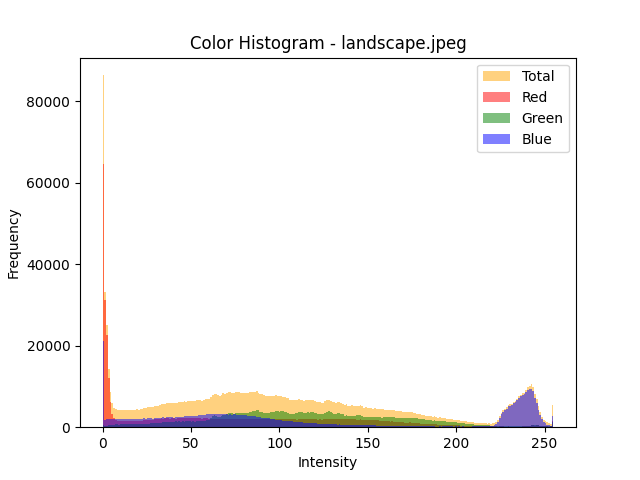
Fig. 8.2 Case_1_Histogram.png

Case 2 Sample Output

$ python3 py4_ind_1_username.py Enter the path of the image folder: grayscale_images grayscale_landscape.jpeg: Brightness: 103.59, Red Content: 0.00

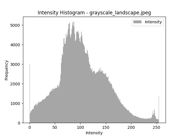
Fig. 8.3 Case_2_Histogram.png

Case 3 Sample Output

$ python3 py4_ind_1_username.py Enter the path of the image folder: empty_images