\[ \begin{align}\begin{aligned}\newcommand\blank{~\underline{\hspace{1.2cm}}~}\\% Bold symbols (vectors) \newcommand\bs[1]{\mathbf{#1}}\\% Poor man's siunitx \newcommand\unit[1]{\mathrm{#1}} \newcommand\num[1]{#1} \newcommand\qty[2]{#1~\unit{#2}}\\\newcommand\per{/} \newcommand\squared{{}^2} \newcommand\cubed{{}^3} % % Scale \newcommand\milli{\unit{m}} \newcommand\centi{\unit{c}} \newcommand\kilo{\unit{k}} \newcommand\mega{\unit{M}} % % Percent \newcommand\percent{\unit{\%}} % % Angle \newcommand\radian{\unit{rad}} \newcommand\degree{\unit{{}^\circ}} % % Time \newcommand\second{\unit{s}} \newcommand\s{\second} \newcommand\minute{\unit{min}} \newcommand\hour{\unit{h}} % % Distance \newcommand\meter{\unit{m}} \newcommand\m{\meter} \newcommand\inch{\unit{in}} \newcommand\foot{\unit{ft}} % % Force \newcommand\newton{\unit{N}} \newcommand\kip{\unit{kip}} % kilopound in "freedom" units - edit made by Sri % % Mass \newcommand\gram{\unit{g}} \newcommand\g{\gram} \newcommand\kilogram{\unit{kg}} \newcommand\kg{\kilogram} \newcommand\grain{\unit{grain}} \newcommand\ounce{\unit{oz}} % % Temperature \newcommand\kelvin{\unit{K}} \newcommand\K{\kelvin} \newcommand\celsius{\unit{{}^\circ C}} \newcommand\C{\celsius} \newcommand\fahrenheit{\unit{{}^\circ F}} \newcommand\F{\fahrenheit} % % Area \newcommand\sqft{\unit{sq\,\foot}} % square foot % % Volume \newcommand\liter{\unit{L}} \newcommand\gallon{\unit{gal}} % % Frequency \newcommand\hertz{\unit{Hz}} \newcommand\rpm{\unit{rpm}} % % Voltage \newcommand\volt{\unit{V}} \newcommand\V{\volt} \newcommand\millivolt{\milli\volt} \newcommand\mV{\milli\volt} \newcommand\kilovolt{\kilo\volt} \newcommand\kV{\kilo\volt} % % Current \newcommand\ampere{\unit{A}} \newcommand\A{\ampere} \newcommand\milliampereA{\milli\ampere} \newcommand\mA{\milli\ampere} \newcommand\kiloampereA{\kilo\ampere} \newcommand\kA{\kilo\ampere} % % Resistance \newcommand\ohm{\Omega} \newcommand\milliohm{\milli\ohm} \newcommand\kiloohm{\kilo\ohm} % correct SI spelling \newcommand\kilohm{\kilo\ohm} % "American" spelling used in siunitx \newcommand\megaohm{\mega\ohm} % correct SI spelling \newcommand\megohm{\mega\ohm} % "American" spelling used in siunitx % % Inductance \newcommand\henry{\unit{H}} \newcommand\H{\henry} \newcommand\millihenry{\milli\henry} \newcommand\mH{\milli\henry} % % Power \newcommand\watt{\unit{W}} \newcommand\W{\watt} \newcommand\milliwatt{\milli\watt} \newcommand\mW{\milli\watt} \newcommand\kilowatt{\kilo\watt} \newcommand\kW{\kilo\watt} % % Energy \newcommand\joule{\unit{J}} \newcommand\J{\joule} % % Composite units % % Torque \newcommand\ozin{\unit{\ounce}\,\unit{in}} \newcommand\newtonmeter{\unit{\newton\,\meter}} % % Pressure \newcommand\psf{\unit{psf}} % pounds per square foot \newcommand\pcf{\unit{pcf}} % pounds per cubic foot \newcommand\pascal{\unit{Pa}} \newcommand\Pa{\pascal} \newcommand\ksi{\unit{ksi}} % kilopound per square inch \newcommand\bar{\unit{bar}} \end{aligned}\end{align} \]

Dec 03, 2024 | 421 words | 4 min read

15.3.2. Task 2

Learning Objectives

Read CSV data in MATLAB and plot data using regression in MATLAB.

Introduction

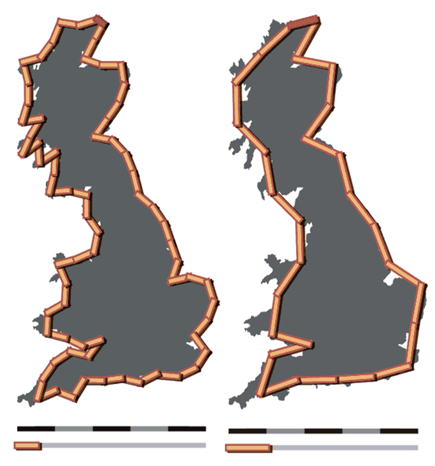
Fig. 15.9 Measurements of Great Britain’s Coastline. CC BY-SA 3.0, sources: 1 2

In the 1950s, Lewis Richardson was trying to determine if there is a relationship between countries’ border lengths and the probability of war. During his research, he noticed that the reported length of borders varied widely between sources. The prevailing method for measuring borders (or coastlines) was to take segments of equal length \(L\) and lay them on a map or photograph and then record the total length of the segments. However, Richardson noticed that using smaller and smaller segment lengths resulted in longer and longer total coastline results. In some cases, it is even true that as \(L\) approaches zero, the length of the coastline approaches infinity. This is now known as the Coastline Paradox. This phenomenon is a result of the fractal-like nature of coastlines, and it also applications in image analysis, acoustics, and material science. In this task you will find an equation that models the relationship between scale and coastline length by using a linear regression

Task Instructions

1. Draft a flowchart for this task and save it as ma4_ind_username.pdf.

2. Open the ENGR133_MATLAB_Template.m MATLAB template and complete the header information. Save your script as ma4_ind_2_username.m

3. Import the data from the coastline.csv file. There are two columns of data in the file. The first contains the scale length (in \(\kilo\meter\)) used to measure the coastline. The second contains the measured length of the coastline (in \(\kilo\meter\)).

4. Using the data you imported, make four subplots in one figure of scale length versus coast length as described below. Be sure to plot the data as points and to format your plots for professional presentation.

   1. Plot 1: both axes are linear

   2. Plot 2: x-axis is logarithmic, y-axis is linear

   3. Plot 3: x-axis is linear, y-axis is logarithmic

   4. Plot 4: both axes are logarithmic

5. Determine which plot makes the data appear most linear. Use polyfit to perform a linear regression on the and plot the regression line with the data on the plot that you chose.

   Hint

   If data appear most linear on the semi-log or log-log plots, you will need to appropriately transform the data before entering it in polyfit. For more help, review the Non-Linear Regression video.

6. Use your model to determine the length of the coastline if it were measured at a \(\qty{100}{\kilo\meter}\) scale, a \(\qty{50}{\kilo\meter}\) scale, and a \(\qty{.001}{\kilo\meter}\) scale.

7. Create an appropriately formatted output that displays the equation of your regression line, and the results of your calculations from step 5.

8. Publish your script as a PDF and name it ma4_ind_1_username.pdf.

9. Upload all your deliverables to Gradescope.

Sample Output

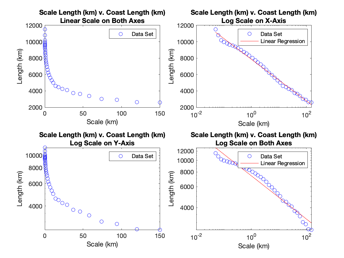
Fig. 15.10 Sample Output for the four plots