\[ \begin{align}\begin{aligned}\newcommand\blank{~\underline{\hspace{1.2cm}}~}\\% Bold symbols (vectors)
\newcommand\bs[1]{\mathbf{#1}}\\% Poor man's siunitx
\newcommand\unit[1]{\mathrm{#1}}
\newcommand\num[1]{#1}
\newcommand\qty[2]{#1~\unit{#2}}\\\newcommand\per{/}
\newcommand\squared{{}^2}
\newcommand\cubed{{}^3}
%
% Scale
\newcommand\milli{\unit{m}}
\newcommand\centi{\unit{c}}
\newcommand\kilo{\unit{k}}
\newcommand\mega{\unit{M}}
%
% Percent
\newcommand\percent{\unit{\%}}
%
% Angle
\newcommand\radian{\unit{rad}}
\newcommand\degree{\unit{{}^\circ}}
%
% Time
\newcommand\second{\unit{s}}
\newcommand\s{\second}
\newcommand\minute{\unit{min}}
\newcommand\hour{\unit{h}}
%
% Distance
\newcommand\meter{\unit{m}}
\newcommand\m{\meter}
\newcommand\inch{\unit{in}}
\newcommand\foot{\unit{ft}}
%
% Force
\newcommand\newton{\unit{N}}
\newcommand\kip{\unit{kip}} % kilopound in "freedom" units - edit made by Sri
%
% Mass
\newcommand\gram{\unit{g}}
\newcommand\g{\gram}
\newcommand\kilogram{\unit{kg}}
\newcommand\kg{\kilogram}
\newcommand\grain{\unit{grain}}
\newcommand\ounce{\unit{oz}}
%
% Temperature
\newcommand\kelvin{\unit{K}}
\newcommand\K{\kelvin}
\newcommand\celsius{\unit{{}^\circ C}}
\newcommand\C{\celsius}
\newcommand\fahrenheit{\unit{{}^\circ F}}
\newcommand\F{\fahrenheit}
%
% Area
\newcommand\sqft{\unit{sq\,\foot}} % square foot
%
% Volume
\newcommand\liter{\unit{L}}
\newcommand\gallon{\unit{gal}}
%
% Frequency
\newcommand\hertz{\unit{Hz}}
\newcommand\rpm{\unit{rpm}}
%
% Voltage
\newcommand\volt{\unit{V}}
\newcommand\V{\volt}
\newcommand\millivolt{\milli\volt}
\newcommand\mV{\milli\volt}
\newcommand\kilovolt{\kilo\volt}
\newcommand\kV{\kilo\volt}
%
% Current
\newcommand\ampere{\unit{A}}
\newcommand\A{\ampere}
\newcommand\milliampereA{\milli\ampere}
\newcommand\mA{\milli\ampere}
\newcommand\kiloampereA{\kilo\ampere}
\newcommand\kA{\kilo\ampere}
%
% Resistance
\newcommand\ohm{\Omega}
\newcommand\milliohm{\milli\ohm}
\newcommand\kiloohm{\kilo\ohm} % correct SI spelling
\newcommand\kilohm{\kilo\ohm} % "American" spelling used in siunitx
\newcommand\megaohm{\mega\ohm} % correct SI spelling
\newcommand\megohm{\mega\ohm} % "American" spelling used in siunitx
%
% Inductance
\newcommand\henry{\unit{H}}
\newcommand\H{\henry}
\newcommand\millihenry{\milli\henry}
\newcommand\mH{\milli\henry}
%
% Power
\newcommand\watt{\unit{W}}
\newcommand\W{\watt}
\newcommand\milliwatt{\milli\watt}
\newcommand\mW{\milli\watt}
\newcommand\kilowatt{\kilo\watt}
\newcommand\kW{\kilo\watt}
%
% Energy
\newcommand\joule{\unit{J}}
\newcommand\J{\joule}
%
% Composite units
%
% Torque
\newcommand\ozin{\unit{\ounce}\,\unit{in}}
\newcommand\newtonmeter{\unit{\newton\,\meter}}
%
% Pressure
\newcommand\psf{\unit{psf}} % pounds per square foot
\newcommand\pcf{\unit{pcf}} % pounds per cubic foot
\newcommand\pascal{\unit{Pa}}
\newcommand\Pa{\pascal}
\newcommand\ksi{\unit{ksi}} % kilopound per square inch
\newcommand\bar{\unit{bar}}
\end{aligned}\end{align} \]
Dec 03, 2024 | 201 words | 2 min read
14.1.2. Task 0
Learning Objectives
Create simple UDF’s in MATLAB . Practice writing a UDF in the same file as the main script and calling the respective function in the main script. Create a simple plot in MATLAB .
Task Instructions
In this task, you will be writing a simple UDF in MATLAB and learning how to create a simple plot.
Make a copy of the ENGR133_MATLAB_Template.m MATLAB template and rename the file to ma3_pre_1_username.m .
Make sure to fill out all header information, including a short description of the code.
In the Initialization Section, initialize the variable, x
Hint
Use the linspace () MATLAB to do this.
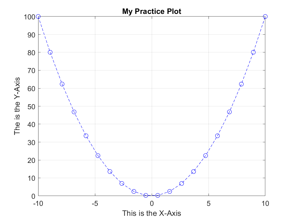
Next, initialize the variable, y, to be \(x^2\) .
In the Outputs Section, create a user-defined function that takes in two variables, x and y, and returns nothing.
In the user-defined function plot the two variables x and y. When plotting the variables, make the line blue with
dashes and circles as the markers.
Title the plot, “My Practice Plot”, and make sure to label the x-axis and y-axis. Also turn the grid on for the
plot.
In the Calculations Section, call the user-defined function with the x and y variables.
Publish your file as ma3_pre_1_username.pdf .
Below is what your plot should look like.