\[ \begin{align}\begin{aligned}\newcommand\blank{~\underline{\hspace{1.2cm}}~}\\% Bold symbols (vectors) \newcommand\bs[1]{\mathbf{#1}}\\% Poor man's siunitx \newcommand\unit[1]{\mathrm{#1}} \newcommand\num[1]{#1} \newcommand\qty[2]{#1~\unit{#2}}\\\newcommand\per{/} \newcommand\squared{{}^2} \newcommand\cubed{{}^3} % % Scale \newcommand\milli{\unit{m}} \newcommand\centi{\unit{c}} \newcommand\kilo{\unit{k}} \newcommand\mega{\unit{M}} % % Percent \newcommand\percent{\unit{\%}} % % Angle \newcommand\radian{\unit{rad}} \newcommand\degree{\unit{{}^\circ}} % % Time \newcommand\second{\unit{s}} \newcommand\s{\second} \newcommand\minute{\unit{min}} \newcommand\hour{\unit{h}} % % Distance \newcommand\meter{\unit{m}} \newcommand\m{\meter} \newcommand\inch{\unit{in}} \newcommand\foot{\unit{ft}} % % Force \newcommand\newton{\unit{N}} \newcommand\kip{\unit{kip}} % kilopound in "freedom" units - edit made by Sri % % Mass \newcommand\gram{\unit{g}} \newcommand\g{\gram} \newcommand\kilogram{\unit{kg}} \newcommand\kg{\kilogram} \newcommand\grain{\unit{grain}} \newcommand\ounce{\unit{oz}} % % Temperature \newcommand\kelvin{\unit{K}} \newcommand\K{\kelvin} \newcommand\celsius{\unit{{}^\circ C}} \newcommand\C{\celsius} \newcommand\fahrenheit{\unit{{}^\circ F}} \newcommand\F{\fahrenheit} % % Area \newcommand\sqft{\unit{sq\,\foot}} % square foot % % Volume \newcommand\liter{\unit{L}} \newcommand\gallon{\unit{gal}} % % Frequency \newcommand\hertz{\unit{Hz}} \newcommand\rpm{\unit{rpm}} % % Voltage \newcommand\volt{\unit{V}} \newcommand\V{\volt} \newcommand\millivolt{\milli\volt} \newcommand\mV{\milli\volt} \newcommand\kilovolt{\kilo\volt} \newcommand\kV{\kilo\volt} % % Current \newcommand\ampere{\unit{A}} \newcommand\A{\ampere} \newcommand\milliampereA{\milli\ampere} \newcommand\mA{\milli\ampere} \newcommand\kiloampereA{\kilo\ampere} \newcommand\kA{\kilo\ampere} % % Resistance \newcommand\ohm{\Omega} \newcommand\milliohm{\milli\ohm} \newcommand\kiloohm{\kilo\ohm} % correct SI spelling \newcommand\kilohm{\kilo\ohm} % "American" spelling used in siunitx \newcommand\megaohm{\mega\ohm} % correct SI spelling \newcommand\megohm{\mega\ohm} % "American" spelling used in siunitx % % Inductance \newcommand\henry{\unit{H}} \newcommand\H{\henry} \newcommand\millihenry{\milli\henry} \newcommand\mH{\milli\henry} % % Power \newcommand\watt{\unit{W}} \newcommand\W{\watt} \newcommand\milliwatt{\milli\watt} \newcommand\mW{\milli\watt} \newcommand\kilowatt{\kilo\watt} \newcommand\kW{\kilo\watt} % % Energy \newcommand\joule{\unit{J}} \newcommand\J{\joule} % % Composite units % % Torque \newcommand\ozin{\unit{\ounce}\,\unit{in}} \newcommand\newtonmeter{\unit{\newton\,\meter}} % % Pressure \newcommand\psf{\unit{psf}} % pounds per square foot \newcommand\pcf{\unit{pcf}} % pounds per cubic foot \newcommand\pascal{\unit{Pa}} \newcommand\Pa{\pascal} \newcommand\ksi{\unit{ksi}} % kilopound per square inch \newcommand\bar{\unit{bar}} \end{aligned}\end{align} \]

Oct 24, 2024 | 969 words | 10 min read

14.3.2. Task 2

Learning Objectives

Learn and practice how to import data, write and run user-defined functions, and plot in MATLAB.

Introduction

Baking, beverage, confectionary, and other food industries sometimes sweeten their products with a mix of glucose and fructose called invert sugar. Invert sugar is liquid and can minimize sugar crystallization within the final products. Invert sugar is made through a process called sugar inversion, where the sucrose in sugar converts into simpler glucose and fructose in the presence of acid and water.

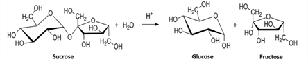
You work for a sweetener company as a food science engineer. You are on a team studying the effect that pH has on sucrose decomposition during sugar inversion and developed a mathematical model for the process. To develop the model, your team ran the same experiment three times, each time adding a sucrose solution to an acid solution and measuring the molar concentration of sucrose every 5 minutes for 60 minutes as the sucrose decomposed into simpler sugars. One teammate found an equation for the mathematical model for the sucrose decomposition in this acidic solution:

\[C = 0.5867e^{-0.060t}\]

Where \(C\) is the molar concentration of sucrose in the solution and \(t\) is elapsed time in minutes. The data for this experiment is in the file Sucrose_Data.csv.

You and your teammates are preparing a presentation of the results. Your responsibility is to prepare plots of the data and model equation for technical presentation. You must plot the appropriate independent and dependent variables on the proper axes and ensure that each figure meets professional plot display expectations. You must perform requested calculations and display their results. Use professional communication standards for all written results and answers.

Your teammates need to be able to understand and run your script, so it must follow good programming standards.

Task Instructions

You will write a script that will create two figures and display some calculated results for your team’s presentation. Follow the steps below.

1. Read the following instructions, then draft a flowchart for this task and save it as ma3_ind_2_flowchart_username.pdf.

2. Open the template (MA3_Task2_sugar_template.m) and complete the header information. Save your script as ma3_ind_2_sugar_username.m.

3. Open the data file Sucrose_Data.csv and review the information it contains.

4. In the INITIALIZATION section of the script:

   • Import the data into the script. Assign each column of data to an appropriately named variable.

   • Generate the vectors needed to plot the mathematical model.

5. Open the MATLAB UDF Template (ENGR133_MATLAB_UDF_Template.m) and fill out the header information for a user-defined function that calculates the average rate of change in sucrose concentration per minute for the first 10 minutes.

   • Create a UDF named ma3_ind_2_secantline_username.m that calculates the slope of the secant line between two points.

   • Your UDF should take in a time vector, a sucrose concentration vector, and the indices of the data that will be used to calculate the secant line.

   • Your UDF should output the slope of the secant line.

   • Do not hard code any data values into your UDF. It should use vector indexing based on the function inputs.

6. In the CALCULATIONS section of the script:

   • Find the mean sucrose concentration at each time in the experiment.

   • Find the standard deviation of the sucrose concentrations at each time in the experiment. (Note: Use a weight of 0 in the standard deviation command)

   • Use the UDF you created to calculate the average rate of change for the mathematical model and each of the three tests using the data point for 1 minute and 10 minutes. (You will need to use your UDF more than once to do this. Do not hard code any data.)

7. In the FIGURE DISPLAY section of the script:

   • Create one figure that displays the following information on one set of axes:

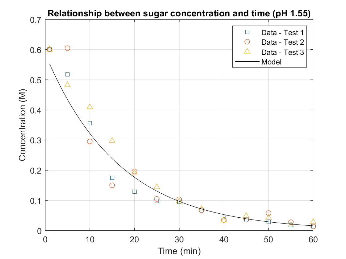
     1. The original data of the sucrose decomposition process for each test.

     2. The team’s model of the sucrose decomposition using a smooth, continuous line.

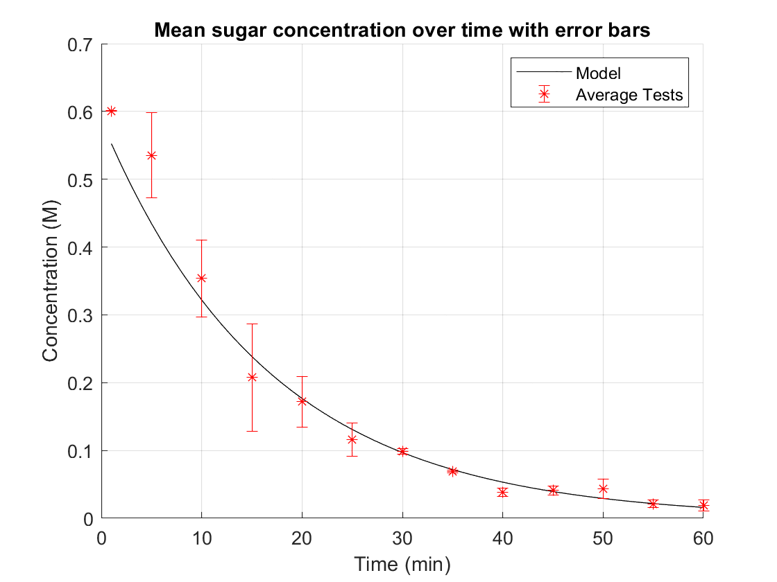
   • Create a second professionally formatted figure that displays the model line, the mean sucrose concentration for the set of experiments, and error bars using the standard deviation.

     1. Display the model line using the plot() command, but you will need to display the mean sucrose concentration values with the error bars using the errorbars() command. It is a specialized plotting command that allows you to plot x-y points with a defined error bar centered on each point. The command requires the x-values as the first input, the y-values as the second input, and the error bar definition as the third input. The final component is the marker specification, just like in the plot() command. In this problem, the proper syntax is errorbar(time, mean_concentration_vec, standard_dev_vec, 'r*').

     • time is your vector of time values

     • mean_concentration_vec is your vector of mean sucrose concentrations, and

     • standard_dev_vec is your vector of the standard deviation values.

     2. All the plot formatting commands will work and should be used to format this figure.

   • Format your plot for professional presentation. Add a descriptive title, axis labels with units, and gridlines for each subplot.

8. In the TEXT DISPLAY section of the script, display the average rates of change from all four calculations above using professional language and formatting. Label them appropriately. Manage your decimal points appropriately. Unsuppressed variable commands are not formatted text displays.

9. Publish your script as a PDF and name it ma3_ind_2_username.pdf.

10. Upload all your deliverables to Gradescope. Answer the following questions in Gradescope.

    a. Do you feel like the model is a good representation of the initial sucrose decomposition process from 1 to 10 minutes? Justify your answer with evidence from your calculations or plots.

    b. One of the primary reasons you created Figures 1 and 2 is to demonstrate how well the model describes the data. Give one example of how Figure 1 is helpful in that demonstration. Give one example of how Figure 2 is helpful.

    c. This experiment was conducted in triplicate (i.e., the same test was run three times). What does your collected data tell you about the consistency of the sucrose decomposition process in the first 10 minutes versus the last 30 minutes? Justify your answer with evidence from your calculations or plots.

Below is a sample output of the two plots for this task.