\[ \begin{align}\begin{aligned}\newcommand\blank{~\underline{\hspace{1.2cm}}~}\\% Bold symbols (vectors) \newcommand\bs[1]{\mathbf{#1}}\\% Poor man's siunitx \newcommand\unit[1]{\mathrm{#1}} \newcommand\num[1]{#1} \newcommand\qty[2]{#1~\unit{#2}}\\\newcommand\per{/} \newcommand\squared{{}^2} \newcommand\cubed{{}^3} % % Scale \newcommand\milli{\unit{m}} \newcommand\centi{\unit{c}} \newcommand\kilo{\unit{k}} \newcommand\mega{\unit{M}} % % Percent \newcommand\percent{\unit{\%}} % % Angle \newcommand\radian{\unit{rad}} \newcommand\degree{\unit{{}^\circ}} % % Time \newcommand\second{\unit{s}} \newcommand\s{\second} \newcommand\minute{\unit{min}} \newcommand\hour{\unit{h}} % % Distance \newcommand\meter{\unit{m}} \newcommand\m{\meter} \newcommand\inch{\unit{in}} \newcommand\foot{\unit{ft}} % % Force \newcommand\newton{\unit{N}} \newcommand\kip{\unit{kip}} % kilopound in "freedom" units - edit made by Sri % % Mass \newcommand\gram{\unit{g}} \newcommand\g{\gram} \newcommand\kilogram{\unit{kg}} \newcommand\kg{\kilogram} \newcommand\grain{\unit{grain}} \newcommand\ounce{\unit{oz}} % % Temperature \newcommand\kelvin{\unit{K}} \newcommand\K{\kelvin} \newcommand\celsius{\unit{{}^\circ C}} \newcommand\C{\celsius} \newcommand\fahrenheit{\unit{{}^\circ F}} \newcommand\F{\fahrenheit} % % Area \newcommand\sqft{\unit{sq\,\foot}} % square foot % % Volume \newcommand\liter{\unit{L}} \newcommand\gallon{\unit{gal}} % % Frequency \newcommand\hertz{\unit{Hz}} \newcommand\rpm{\unit{rpm}} % % Voltage \newcommand\volt{\unit{V}} \newcommand\V{\volt} \newcommand\millivolt{\milli\volt} \newcommand\mV{\milli\volt} \newcommand\kilovolt{\kilo\volt} \newcommand\kV{\kilo\volt} % % Current \newcommand\ampere{\unit{A}} \newcommand\A{\ampere} \newcommand\milliampereA{\milli\ampere} \newcommand\mA{\milli\ampere} \newcommand\kiloampereA{\kilo\ampere} \newcommand\kA{\kilo\ampere} % % Resistance \newcommand\ohm{\Omega} \newcommand\milliohm{\milli\ohm} \newcommand\kiloohm{\kilo\ohm} % correct SI spelling \newcommand\kilohm{\kilo\ohm} % "American" spelling used in siunitx \newcommand\megaohm{\mega\ohm} % correct SI spelling \newcommand\megohm{\mega\ohm} % "American" spelling used in siunitx % % Inductance \newcommand\henry{\unit{H}} \newcommand\H{\henry} \newcommand\millihenry{\milli\henry} \newcommand\mH{\milli\henry} % % Power \newcommand\watt{\unit{W}} \newcommand\W{\watt} \newcommand\milliwatt{\milli\watt} \newcommand\mW{\milli\watt} \newcommand\kilowatt{\kilo\watt} \newcommand\kW{\kilo\watt} % % Energy \newcommand\joule{\unit{J}} \newcommand\J{\joule} % % Composite units % % Torque \newcommand\ozin{\unit{\ounce}\,\unit{in}} \newcommand\newtonmeter{\unit{\newton\,\meter}} % % Pressure \newcommand\psf{\unit{psf}} % pounds per square foot \newcommand\pcf{\unit{pcf}} % pounds per cubic foot \newcommand\pascal{\unit{Pa}} \newcommand\Pa{\pascal} \newcommand\ksi{\unit{ksi}} % kilopound per square inch \newcommand\bar{\unit{bar}} \end{aligned}\end{align} \]

Oct 24, 2024 | 693 words | 7 min read

14.2.3. Task 3

Learning Objectives

Create user defined functions in MATLAB. Create plots in MATLAB.

Introduction

Energy conversion is a concern for many engineering disciplines. For example, heating, ventilation, and air conditioning (HVAC) requires an engineer to understand how heat flows in and out of a building. One way that heat interacts with a building in through windows. Solar radiation enters the building through windows. Horizontal blinds on a window can control how much solar radiation passes through.

Horizontal blinds transmit, absorb, and reflect solar radiation, and these radiation values can be calculated. The calculations require knowledge of the operational geometry of a horizontal blind, as shown in Figure 2.

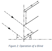
The geometric parameters of a blind are:

• \(W\) = slat width (mm)

• \(S\) = slat spacing (mm)

• \(M\) = width of slat that is illuminated (mm)

• \(\sigma\) = vertical shadow angle (given in degrees)

• \(\Psi\) = slat angle with horizontal (given in degrees)

• Additionally, the blind surface material has an absorptivity constant, \(a\) (alpha). This is a dimensionless value between 0-1.

When the slats of the blind are fully illuminated (i.e., when \(M\) = \(W\)) by incoming light, there are three fractions that are used in the transmission and absorption equations:

\(F_1\): Fraction of total radiation reflected by the lower slat that passed into the room when the whole width of a slat is illuminated.

\[F_1=\frac{1}{2}\left( 1 + \frac{S}{W} - \sqrt[]{1 + \left(\frac{S}{W}\right)^{2} + 2\frac{S}{W}sin(\Psi)}\right)\]

\(F_2\): Fraction of total radiation reflected by the lower slat that is intercepted by the upper slat when the whole width is illuminated.

\[F_2 = \frac{1}{2}\left( \sqrt{1 + \left( \frac{S}{W} \right)^2 + 2\frac{S}{W}sin(\Psi)} +\sqrt{1 + \left( \frac{S}{W} \right)^2 - 2\frac{S}{W}sin(\Psi)} -2\frac{S}{W}\right)\]

\(F_3\): Fraction of radiation reflected by the upper slat that passes into the room.

\[F_3 = \frac{1}{2}\left( 1 + \frac{S}{W} -\sqrt{1 + \left( \frac{S}{W} \right)^2 - 2\frac{S}{W}sin(\Psi)} \right)\]

With the fraction results, you can use the following equations to determine the total fraction of radiation transmitted, absorbed, and reflected by the blinds when the blind slats are fully illuminated.

The total fraction of radiation transmitted by the blind is

\[T_D = 1 - \frac{W}{S}\frac{sin(\sigma+\Psi)}{cos(\sigma)}\left( 1 - F_1(1-a) - \frac{F_2(1-a)^2[F_3+F_1\cdot F_2(1-a)]}{1-F_2^2(1-a)^2)} \right)\]

The total fraction of radiation absorbed is

\[A_D =\frac{aWsin(\sigma+\Psi)}{Scos(\sigma)[1-F_2(1-a)]}\]

Task Instructions

You are given the parameters for a specific set of binds (Table ). You will write and use user-defined functions to calculate the transmission and absorption values for three settings of the blind (Table 2).

Table 14.6 Table 1: Blind Parameters

Blind Parameters
Slat Spacing (\(S\))	50 mm
Slat Width (\(W)\)	60 mm
Absorptivity Constant (\(a\))	0.76
Shadow Angle (\(\sigma\))	45 degrees

Table 14.7 Table 2: Blind Settings

Parameter	Slat Angle with the Horizontal (\(\Psi\))
Setting 1	30 degrees
Setting 2	45 degrees
Setting 3	60 degrees

Part A

1. Draft a flowchart for this task and save it in the already created pdf, ma3_team_teamnumber.pdf.

2. Open the MATLAB Template ENGR133_MATLAB_Template.m and fill out the header information. Write a script named ma3_team_3_partA_teamnumber.m that:

   • Initializes the given values of the blind parameters from Table 1 under INTIALIZATION.

   • Calls the user-defined functions created in Task 2 under CALCULATIONS.

   • Prints the results from the transmission and absorption UDFs to the command window under OUTPUTS for all three blind settings.

   Hint

   Use a for loop.

Sample Output

Use the values in Table 14.8 below to test your program.

Table 14.8 Test Cases

Case
1

Ensure your program’s output matches the provided samples exactly. This includes all characters, white space, and punctuation. In the samples, user input is highlighted like this for clarity, but your program should not highlight user input in this way.

Case 1 Sample Output

>> ma3_team_3_a_teamnumber The transmission value for Blind 1 at angle 30.0 is -0.57. The absorption value for Blind 1 at angle 30.0 is 1.39.

The transmission value for Blind 1 at angle 45.0 is -0.65. The absorption value for Blind 1 at angle 45.0 is 1.42.

The transmission value for Blind 1 at angle 60.0 is -0.61. The absorption value for Blind 1 at angle 60.0 is 1.34.

Part B

1. Draft a flowchart for this task and save it in the already created pdf, ma3_team_teamnumber.pdf.

2. Open the MATLAB Template ENGR133_MATLAB_Template.m and fill out the header information. Write a script named ma3_team_3_partB_teamnumber.m that: (This will be similar to Part A, so it will benefit your team to do Part A together first.)

   • Initializes the given values of the blind parameters from the MA3_Blind_Settings_Data.csv under INTIALIZATION. The slat angle with the horizontal will be a vector of the entire last row.

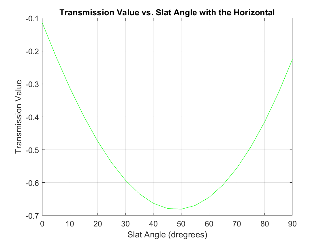
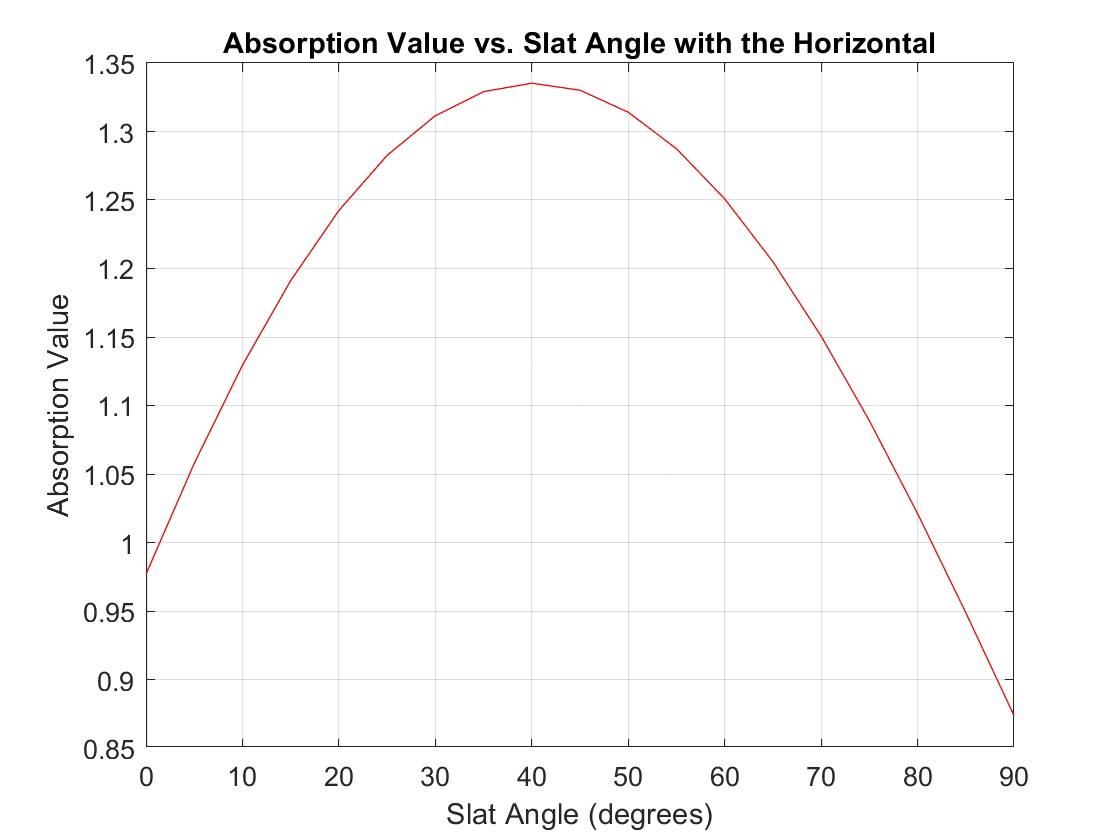
   • Loops through all the values for the slat angle with the horizontal and calculates the total fraction of radiation transmitted by the blind and the total fraction of radiation absorbed by the blind using the user-defined functions created in Task 2 under CALCULATIONS. Make sure to save the calculated values for Transmission and Absorption to a vector.

   • Uses the plotting function made in the Pre-Class Task 0 to plot the Absorption Value vs. Slat Angle with the Horizontal and the Transmission Value vs. Slat Angle with the Horizontal under the OUTPUTS section. You may want to add more arguments to your plotting function so that the function can take in strings for the title, x-axis label, y-axis label, and color. The plotting function can be copy and pasted into the bottom of your MATLAB file.

Below is a sample output of the two plots for this task.